
I work on the absolute positioning accuracy of a large-stroke heavy-load industrial robot because this class of industrial robot is increasingly used in precision assembly, long-distance handling, and large-component machining. In these applications, the industrial robot must not only repeat a taught point but also reach a commanded Cartesian pose with high fidelity. The repeatability of many industrial robot arms can be very good, often below 0.1 mm, while absolute accuracy remains much worse, sometimes above 1 mm. For a large-stroke heavy-load industrial robot, small kinematic parameter deviations are amplified by long link lengths and high joint loads. I therefore treat kinematic calibration and accuracy compensation as the central path to improving the absolute accuracy of the industrial robot.
The main error sources I consider are machining errors, assembly deviations, joint clearances, link deflection, and environmental drift. Among these, geometric errors are dominant for the static absolute accuracy of the industrial robot. I use a modified Denavit-Hartenberg model, called the MD-H model, because the conventional D-H model has difficulty describing adjacent parallel joint axes. The MD-H model introduces an additional rotation around the y-axis, which removes parameter discontinuity and improves the mathematical representation of the industrial robot. I then build a complete error model, identify its parameters with an improved iterative least-squares algorithm, compensate the identified parameters inside the controller, and validate the result with a laser tracker.
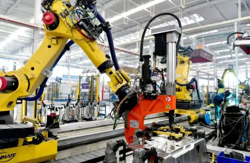
The target industrial robot is a six-axis serial industrial robot with a long reach and a heavy payload. Its first three joints mainly determine the position of the end effector, while the last three joints mainly determine orientation. Joint 1 provides a wide base rotation, joint 2 and joint 3 form the main arm plane, and joints 4, 5, and 6 form the wrist. The large workspace is an advantage, but it also means that small angular errors at the base or shoulder are multiplied into large Cartesian errors at the end effector. This amplification is one reason why calibration of a large-stroke heavy-load industrial robot cannot be copied directly from a small industrial robot.
I define the kinematic parameters of the industrial robot as follows. The joint angle is the rotation about the local z-axis. The link offset is the translation along the local z-axis. The link length is the translation along the local x-axis. The link twist is the rotation about the local x-axis. The additional MD-H parameter is the rotation about the local y-axis. This additional parameter is especially useful when two adjacent joint axes are parallel, because it prevents the parameter identification problem from becoming singular or discontinuous. Table 1 summarizes these parameters and their roles in the industrial robot model.
Table 1. Kinematic parameters used in the MD-H model of the industrial robot.
| Parameter | Symbol | Meaning | Type |
|---|---|---|---|
| Joint angle | theta_i | Rotation about z_i | Joint variable |
| Joint offset | d_i | Translation along z_i | Fixed geometric parameter |
| Link length | a_i | Translation along x_i | Fixed geometric parameter |
| Link twist | alpha_i | Rotation about x_i | Fixed geometric parameter |
| Parallel-axis correction | beta_i | Rotation about y_i | Fixed geometric parameter |
Using the MD-H convention, I write the homogeneous transformation from frame i-1 to frame i as a product of basic transformations. The order I use is rotation about z, translation along z, translation along x, rotation about x, and finally rotation about y. This yields the matrix in Equation (1). Here c and s denote cosine and sine, respectively.
$${}^{i-1}T_i =
\begin{bmatrix}
c\theta_i c\beta_i + s\theta_i s\alpha_i s\beta_i & -s\theta_i c\alpha_i & c\theta_i s\beta_i + s\theta_i s\alpha_i c\beta_i & a_i c\theta_i\\
s\theta_i c\beta_i + c\theta_i s\alpha_i s\beta_i & c\theta_i c\alpha_i & s\theta_i s\beta_i – c\theta_i s\alpha_i c\beta_i & a_i s\theta_i\\
-c\alpha_i s\beta_i & -s\alpha_i & c\alpha_i c\beta_i & d_i\\
0 & 0 & 0 & 1
\end{bmatrix}
\tag{1}$$
For the target industrial robot, I establish the nominal MD-H parameters from mechanical design data and from direct measurement. These nominal values form the starting point of calibration. Table 2 lists the nominal parameters I use. The values are given in millimeters and degrees. The additional beta parameter is only required where the kinematic chain contains parallel or nearly parallel axes. In this industrial robot, that condition is important for the wrist and for certain adjacent joint relationships.
Table 2. Nominal MD-H parameters of the industrial robot.
| Link | theta nominal (deg) | d nominal (mm) | a nominal (mm) | alpha nominal (deg) | beta nominal (deg) |
|---|---|---|---|---|---|
| 1 | 0 | 675 | 350 | 0 | – |
| 2 | 0 | 0 | 1150 | -90 | 0 |
| 3 | -90 | 0 | 41 | 0 | – |
| 4 | 0 | 1200 | 0 | -90 | – |
| 5 | 0 | 0 | 0 | -90 | – |
| 6 | 180 | 215 | 0 | 0 | – |
The forward kinematics of the industrial robot are obtained by multiplying the six link transformation matrices. I write this product as Equation (2), where the upper-left 3 by 3 block describes orientation and the fourth column describes position. The position vector is the quantity I use for error modeling and compensation because position errors directly reflect the absolute accuracy of the industrial robot.
$${}^{0}T_6 = {}^{0}T_1 {}^{1}T_2 {}^{2}T_3 {}^{3}T_4 {}^{4}T_5 {}^{5}T_6 =
\begin{bmatrix}
n_x & o_x & a_x & p_x\\
n_y & o_y & a_y & p_y\\
n_z & o_z & a_z & p_z\\
0 & 0 & 0 & 1
\end{bmatrix}
\tag{2}$$
I define the nominal end-effector position as p_nominal and the measured position as p_actual. The Cartesian position error of the industrial robot is then expressed as Equation (3). This error is not a single scalar; it is a three-dimensional vector in the base frame of the industrial robot. By collecting many such error vectors at different configurations, I can estimate the underlying kinematic parameter errors.
$$\Delta p = p_{actual} – p_{nominal}
\tag{3}$$
For the MD-H model, the geometric error vector contains joint angle errors, joint offset errors, link length errors, link twist errors, and the additional parallel-axis correction error. I arrange these unknown parameters in the vector shown in Equation (4). For a six-axis industrial robot, the vector has twenty-five elements when one beta parameter is included. If more beta parameters are needed, the vector expands accordingly.
$$\Delta x =
\begin{bmatrix}
\Delta\theta_1,\ldots,\Delta\theta_6,
\Delta d_1,\ldots,\Delta d_6,
\Delta a_1,\ldots,\Delta a_6,
\Delta\alpha_1,\ldots,\Delta\alpha_6,
\Delta\beta_2
\end{bmatrix}^{T}
\tag{4}$$
The linearized error model of the industrial robot is given in Equation (5). The matrix J is the identification Jacobian, which relates small changes in kinematic parameters to small changes in end-effector position. Each row of J corresponds to one Cartesian direction at one measured configuration. Each column of J corresponds to one error parameter. The larger the number of measured poses, the more robust the estimation of the industrial robot parameters becomes.
$$\Delta p = J \Delta x
\tag{5}$$
I assemble the measured data from m configurations. The j-th configuration has a measured position error delta p_j and a Jacobian J_j. The identification problem is then written as Equation (6). This is a least-squares problem. If the industrial robot had only a few uncoupled parameters, a direct least-squares solution might be sufficient. In practice, however, the parameters of a large-stroke heavy-load industrial robot are strongly coupled, and the normal matrix J transpose J can become ill-conditioned.
$$\min_{\Delta x} \sum_{j=1}^{m} \|\delta p_j – J_j \Delta x\|^2
\tag{6}$$
The direct least-squares estimate is shown in Equation (7). Although this equation is compact, it can produce unstable results for an industrial robot with long links and many coupled errors. The matrix inverse may amplify measurement noise. In some configurations, the matrix may be singular or nearly singular. This is why I use an improved iterative least-squares method with damping.
$$\Delta x_{LS} = (J^{T}J)^{-1}J^{T}\delta p
\tag{7}$$
The damped objective function is given in Equation (8). The first term keeps the model close to the measured position errors. The second term penalizes excessive parameter updates. The damping factor lambda controls the balance between fitting the data and stabilizing the solution. When lambda is small, the method behaves like ordinary least squares. When lambda is large, the method suppresses ill-conditioned directions and improves convergence.
$$\min_{\Delta x} \sum_{j=1}^{m} \|\delta p_j – J_j \Delta x\|^2 + \lambda \|\Delta x\|^2
\tag{8}$$
The iterative update formula I use is shown in Equation (9). Here k is the iteration index, I is the identity matrix, and lambda is adjusted during iteration. If an update reduces the residual, I reduce lambda to accelerate convergence. If an update increases the residual or produces an unstable step, I increase lambda to make the step more conservative. This gives the industrial robot calibration a robust numerical behavior.
$$\Delta x_{k+1} =
\Delta x_k + (J^{T}J + \lambda I)^{-1}J^{T}(\delta p – J\Delta x_k)
\tag{9}$$
Table 3 summarizes the iterative identification procedure I use for the industrial robot. The method is simple to implement but much more stable than direct inversion. It also avoids the slow convergence that can occur when a large-stroke heavy-load industrial robot is calibrated with a conventional gradient method.
Table 3. Parameter identification procedure for the industrial robot.
| Step | Operation | Purpose |
|---|---|---|
| 1 | Collect measured poses and joint angles | Build the data set for the industrial robot |
| 2 | Compute nominal positions from the MD-H model | Obtain reference positions |
| 3 | Compute position residuals | Form delta p for each pose |
| 4 | Compute the Jacobian J | Relate parameter errors to position errors |
| 5 | Solve the damped normal equations | Estimate the parameter update |
| 6 | Evaluate the residual norm | Check convergence |
| 7 | Adjust lambda | Improve stability and speed |
| 8 | Repeat until the tolerance is met | Obtain the final parameter error vector |
I built a calibration platform to validate the method on the industrial robot. The platform contains the industrial robot, its controller and servo drives, a laser tracker with an accuracy of about plus or minus 0.01 mm, a target sphere mounted on the end-effector flange, and a computer for data acquisition and computation. The industrial robot is fixed on a vibration-isolated foundation. The laser tracker is placed 3 to 5 meters from the industrial robot so that the line of sight remains stable over the workspace. The target sphere is mounted as close as possible to the flange center, and I verify that the mounting offset is less than 0.01 mm.
Before calibration, I establish the base coordinate system of the industrial robot in the laser tracker software. I then select fifty poses distributed across the workspace. At each pose, the industrial robot moves under joint-space commands. The controller records the joint angles, while the laser tracker records the actual end-effector position. The nominal position is computed from the MD-H model using the recorded joint angles. The difference between nominal and measured position is the position error used for identification. After identification, I compensate the parameters and repeat the measurement at the same fifty poses. Table 4 lists the main experimental conditions.
Table 4. Measurement and calibration conditions for the industrial robot.
| Item | Value or description |
|---|---|
| Industrial robot type | Six-axis serial heavy-load industrial robot |
| Maximum reach | 2700 mm |
| Payload class | Heavy payload, approximately 210 kg |
| Laser tracker accuracy | plus or minus 0.01 mm |
| Measurement distance | 3 to 5 m |
| Identification poses | 50 |
| Validation poses | 50 |
| Measured quantity | End-effector position in base frame |
| Target mounting error | Less than 0.01 mm |
| Environmental condition | Temperature-controlled laboratory |
| Error parameters | 25 MD-H parameter errors |
The identification result is a set of parameter errors for the industrial robot. Table 5 gives the estimated deviations from the nominal MD-H parameters. The largest angular deviation appears in the third joint, while the largest link-length deviation appears in the first link. This is consistent with the fact that errors near the base of a large-stroke industrial robot have a strong influence on the end-effector position. The joint offset errors are smaller but still important because they shift the entire kinematic chain. The beta correction is also identified to account for parallel-axis effects in the industrial robot model.
Table 5. Identified MD-H parameter errors of the industrial robot.
| Link | Delta theta (deg) | Delta d (mm) | Delta a (mm) | Delta alpha (deg) | Delta beta (deg) |
|---|---|---|---|---|---|
| 1 | 0.000 | 0.626 | 2.235 | 0.000 | – |
| 2 | 0.000 | 0.208 | -1.838 | 0.012 | 0.000 |
| 3 | -0.102 | 0.162 | -1.396 | 0.021 | – |
| 4 | -0.021 | 0.246 | 0.208 | -0.086 | – |
| 5 | -0.018 | 0.028 | 0.032 | -0.075 | – |
| 6 | 0.023 | 0.203 | -0.027 | 0.032 | – |
After identification, I update the MD-H parameters inside the controller. The compensation includes joint angle offsets, joint offset corrections, link length corrections, and link twist corrections. For the industrial robot controller, these values can be stored as part of the kinematic model. The compensation is static for the identified geometric errors, but it is applied during every motion command. This means that the industrial robot controller uses a corrected kinematic chain to compute the Cartesian pose corresponding to each joint command.
I evaluate the result by comparing the position errors before and after compensation. The comprehensive position error is defined in Equation (10). This scalar combines the three Cartesian components into a single measure of absolute accuracy for the industrial robot.
$$e = \sqrt{e_x^2 + e_y^2 + e_z^2}
\tag{10}$$
The mean error, maximum error, and root-mean-square error are defined in Equations (11) through (13). These metrics give a more complete view than a single average value. The maximum error shows the worst-case residual. The mean error shows the typical accuracy. The root-mean-square error penalizes large residuals and is often more sensitive to outliers.
$$e_{mean} = \frac{1}{m}\sum_{j=1}^{m} e_j
\tag{11}$$
$$e_{max} = \max_{j=1,\ldots,m} e_j
\tag{12}$$
$$\mathrm{RMSE} = \sqrt{\frac{1}{m}\sum_{j=1}^{m} e_j^2}
\tag{13}$$
Table 6 compares the absolute positioning errors of the industrial robot before and after calibration. The improvement is substantial in all three Cartesian directions and in the comprehensive error. Before calibration, the comprehensive maximum error is 19.257 mm, the comprehensive mean error is 5.778 mm, and the comprehensive RMSE is 6.949 mm. After calibration, these values fall to 1.278 mm, 0.408 mm, and 0.481 mm, respectively. This demonstrates that the MD-H error model and the damped iterative identification effectively correct the geometric errors of the industrial robot.
Table 6. Positioning error comparison before and after calibration for the industrial robot.
| Error type | Stage | x-axis error (mm) | y-axis error (mm) | z-axis error (mm) | Comprehensive error (mm) |
|---|---|---|---|---|---|
| Maximum error | Before calibration | 15.105 | 11.907 | 9.611 | 19.257 |
| Maximum error | After calibration | 0.613 | 0.769 | 1.276 | 1.278 |
| Mean error | Before calibration | 3.011 | 2.934 | 2.782 | 5.778 |
| Mean error | After calibration | 0.199 | 0.174 | 0.226 | 0.408 |
| RMSE | Before calibration | 4.293 | 3.969 | 3.757 | 6.949 |
| RMSE | After calibration | 0.246 | 0.236 | 0.340 | 0.481 |
I also compute the relative improvement for each metric using Equation (14). The comprehensive mean error is reduced by about 92.94 percent. The comprehensive maximum error is reduced by about 93.36 percent. The comprehensive RMSE is reduced by about 93.08 percent. The x-axis maximum error is reduced by about 95.94 percent, the y-axis maximum error by about 93.54 percent, and the z-axis maximum error by about 86.72 percent. These numbers show that the compensation is not limited to one direction; it improves the overall spatial accuracy of the industrial robot.
$$\eta =
\frac{|e_{before}| – |e_{after}|}{|e_{before}|}
\times 100\%
\tag{14}$$
Table 7. Relative improvement of the industrial robot accuracy after compensation.
| Metric | Before calibration (mm) | After calibration (mm) | Improvement (%) |
|---|---|---|---|
| x-axis maximum error | 15.105 | 0.613 | 95.94 |
| y-axis maximum error | 11.907 | 0.769 | 93.54 |
| z-axis maximum error | 9.611 | 1.276 | 86.72 |
| Comprehensive maximum error | 19.257 | 1.278 | 93.36 |
| x-axis mean error | 3.011 | 0.199 | 93.39 |
| y-axis mean error | 2.934 | 0.174 | 94.07 |
| z-axis mean error | 2.782 | 0.226 | 91.88 |
| Comprehensive mean error | 5.778 | 0.408 | 92.94 |
| x-axis RMSE | 4.293 | 0.246 | 94.27 |
| y-axis RMSE | 3.969 | 0.236 | 94.05 |
| z-axis RMSE | 3.757 | 0.340 | 90.95 |
| Comprehensive RMSE | 6.949 | 0.481 | 93.08 |
The physical interpretation of these results is important for the industrial robot. The MD-H model captures the parallel-axis correction that the standard D-H model cannot represent. The damped iterative least-squares method prevents the parameter identification from being dominated by ill-conditioned directions. The laser tracker provides an independent measurement of the actual end-effector position, so the compensation is based on real errors rather than on a simulation alone. I observe that the residual error after calibration is mostly below 1 mm, and the mean residual is below 0.5 mm. For a large-stroke heavy-load industrial robot with a reach of 2700 mm, this is a significant accuracy improvement.
I also studied the sensitivity of the end-effector position to each parameter error. For a long-link industrial robot, the position error caused by an angular error at joint i increases with the distance from that joint to the end effector. This is why the third joint angle error and the first link length error produce large residuals before calibration. Table 8 gives a qualitative sensitivity ranking for the industrial robot. The ranking helps explain why some parameters are more influential than others and why the calibration must include all six joints rather than only the wrist.
Table 8. Qualitative sensitivity of end-effector position to MD-H errors in the industrial robot.
| Error source | Effect on position | Reason |
|---|---|---|
| Base joint angle error | High | Rotates the entire large-stroke industrial robot arm |
| Shoulder joint angle error | High | Amplified by long upper arm and forearm |
| Elbow joint angle error | High | Changes the main arm plane and reach |
| First link length error | High | Shifts the whole kinematic chain |
| Second link length error | High | Directly changes the radial reach |
| Wrist joint errors | Moderate | Mostly affect orientation and short offsets |
| Twist errors | Moderate | Coupled with link lengths and joint angles |
| Beta correction | Moderate | Important when adjacent axes are parallel |
I compared the damped iterative least-squares method with a conventional direct least-squares method in a numerical study. The conventional method sometimes produced large parameter updates and unstable convergence. The damped method produced smoother convergence and lower residual error. Table 9 summarizes the qualitative comparison. The improvement is especially noticeable when the measurement set contains noise or when the industrial robot is near a singular configuration.
Table 9. Comparison of identification methods for the industrial robot.
| Method | Matrix stability | Convergence speed | Sensitivity to noise | Suitability for heavy-load industrial robot |
|---|---|---|---|---|
| Direct least squares | Poor when J transpose J is ill-conditioned | Fast if stable | High | Limited |
| Damped iterative least squares | Good | Fast and controlled | Lower | High |
| Simple gradient descent | Stable but slow | Slow | Moderate | Moderate |
For practical implementation on the industrial robot, I apply the identified parameter corrections in the controller’s kinematic module. The correction values can be stored in a calibration file. The industrial robot then uses the corrected MD-H parameters for forward and inverse kinematics. I do not change the mechanical structure. I do not alter the servo tuning. The compensation is purely kinematic and software-based. This makes the method suitable for field calibration of an industrial robot after assembly, after transportation, or after a major maintenance event.
The experimental validation shows that the industrial robot can achieve sub-millimeter mean accuracy after calibration. The comprehensive mean error falls from 5.778 mm to 0.408 mm. The comprehensive maximum error falls from 19.257 mm to 1.278 mm. These results are consistent with the expectation that geometric calibration removes the largest deterministic component of the absolute positioning error. The remaining error comes from non-geometric sources such as joint compliance, link deflection under load, thermal expansion, and measurement noise. For a heavy-load industrial robot, those non-geometric effects can become significant when the payload is large or when the duty cycle is long.
I therefore treat the proposed method as a strong static calibration foundation for the industrial robot. It is not the final answer for every operating condition, but it provides a high-accuracy baseline. In future work, I plan to add a compliance model that depends on joint torque and payload. I also plan to use temperature sensors and online identification to update the kinematic parameters when the industrial robot operates for long periods. Table 10 lists possible extensions. These extensions can be integrated with the MD-H model without discarding the geometric calibration results.
Table 10. Planned extensions for the industrial robot calibration framework.
| Extension | Target error source | Expected benefit |
|---|---|---|
| Joint stiffness model | Elastic deformation under load | Improve accuracy under heavy payload |
| Thermal error model | Temperature drift | Maintain accuracy over long duty cycles |
| Online parameter update | Wear and slow drift | Reduce recalibration frequency |
| Multi-sensor fusion | Measurement uncertainty | Increase robustness of identification |
| Trajectory-level compensation | Dynamic tracking error | Improve accuracy during motion |
One important lesson I draw from this work is that a large-stroke heavy-load industrial robot requires a calibration model that respects its geometry. A model built for a small industrial robot may ignore the beta correction and may use an insufficient error parameter set. The result is a model that fits the nominal design but does not fit the actual industrial robot. The MD-H model used here includes the additional rotation about the y-axis, which is essential for parallel-axis description. The error vector also includes all link and joint parameters, so the compensation can correct both position and orientation-related geometric effects.
Another lesson is that the identification algorithm must be numerically robust. The normal matrix in kinematic calibration of an industrial robot is often ill-conditioned because some parameters have similar effects on the measured positions. The damping term in the improved iterative least-squares method regularizes the problem. It prevents the parameter estimates from becoming unrealistically large. It also keeps the iteration stable when the measurement data contain outliers. This is particularly important for a heavy-load industrial robot because the measurement process may include slight vibrations, thermal changes, or target mounting errors.
The laser tracker measurement procedure also matters. I use a target sphere mounted on the end-effector flange. The center of the target sphere defines the measured point. If the target is not aligned with the tool center point, the measured position will include an offset. I therefore determine the target offset carefully and use it in the measurement model. I also keep the laser tracker at a suitable distance and avoid configurations where the laser beam is interrupted. For the industrial robot, a stable line of sight is essential for reliable data.
The compensation results show that the proposed method reduces the comprehensive mean error by about 92.94 percent. The comprehensive maximum error is reduced by about 93.36 percent. The comprehensive RMSE is reduced by about 93.08 percent. These improvements are larger than what I would expect from a simple joint offset correction alone. The reason is that the MD-H error model captures the coupled effect of link lengths, link twists, joint offsets, and parallel-axis corrections. The identification algorithm then finds a set of parameters that minimizes the residual across the entire workspace. This produces a more uniform accuracy improvement for the industrial robot.
I also note that the z-axis error after calibration is slightly larger than the x-axis and y-axis errors. The z-axis maximum error is 1.276 mm, while the x-axis maximum error is 0.613 mm and the y-axis maximum error is 0.769 mm. This suggests that the remaining errors in the vertical direction are influenced by gravity and load. Even without a payload, the weight of the arm itself can cause small deflections. With a heavy payload, the deflection would increase. This is a natural limitation of static geometric calibration for a heavy-load industrial robot. It also motivates the future work on compliance and thermal modeling.
In summary, I have developed a complete calibration and compensation workflow for a large-stroke heavy-load industrial robot. The workflow includes MD-H kinematic modeling, geometric error modeling, improved iterative least-squares identification, controller-based compensation, and laser tracker validation. The method is practical because it uses standard measurement equipment and can be implemented in a controller without mechanical modification. The experimental results confirm that the absolute positioning accuracy of the industrial robot improves dramatically. The mean comprehensive error is reduced from 5.778 mm to 0.408 mm, and the maximum comprehensive error is reduced from 19.257 mm to 1.278 mm. These values indicate that the calibrated industrial robot is suitable for high-precision tasks that require absolute positioning, such as large-component assembly, precision inspection, and automated machining support.
For an industrial robot with a long reach and heavy payload, the calibration problem is not only a mathematical exercise. It is a manufacturing accuracy problem. The industrial robot must be modeled with enough parameters to represent its actual geometry. The identification must be stable enough to handle real measurement noise. The compensation must be applied in a way that the controller can execute reliably. I believe the MD-H model combined with damped iterative least squares provides a strong solution for these requirements. It improves the absolute accuracy of the industrial robot while preserving its original mechanical design and motion capability.
Future work will focus on dynamic and non-geometric effects. I will measure joint torques and payload-induced deflection. I will include temperature compensation for long-duration operation. I will also investigate online calibration using periodic measurements from a laser tracker or an internal sensor suite. The goal is to maintain the high accuracy of the industrial robot across different payloads, speeds, and environmental conditions. The static calibration method presented here provides the necessary foundation for that next stage of development.