
I begin with the observation that industrial robots have become essential in modern manufacturing because they combine repeatability, programmability, and versatility across tasks such as assembly, machining, palletizing, inspection, and material handling. In many of these applications, the absolute positioning accuracy of industrial robots is a decisive performance index, because offline programming and high-precision task execution require the robot controller to predict the true end-effector pose with small uncertainty. For small and medium-sized industrial robots, repeatability is often below 0.1 mm, while absolute accuracy may remain above 1 mm. This gap becomes even more serious for large-stroke heavy-load industrial robots, where small kinematic parameter deviations are amplified by long link lengths and high payloads. Consequently, geometric calibration and accuracy compensation are indispensable for improving the absolute accuracy of industrial robots without modifying their mechanical structure.
I focus on a large-stroke heavy-load industrial robot with a maximum reach of 2700 mm and a rated payload of 210 kg. This class of industrial robots is widely used for handling large components, long-distance transfer, and heavy assembly. However, machining errors, assembly deviations, joint clearances, link deflections, and environmental disturbances cause the actual kinematic parameters to differ from their nominal values. Because the arm is long, even a small angular error at the base or shoulder joint can produce a large positional deviation at the end effector. Therefore, I develop a complete kinematic calibration and compensation method based on a modified Denavit–Hartenberg (MD-H) model. The method includes kinematic modeling, geometric error modeling, parameter identification with an improved iterative least-squares algorithm, and experimental validation with a laser tracker.
The physical structure and dimensional layout of the industrial robot are illustrated below.
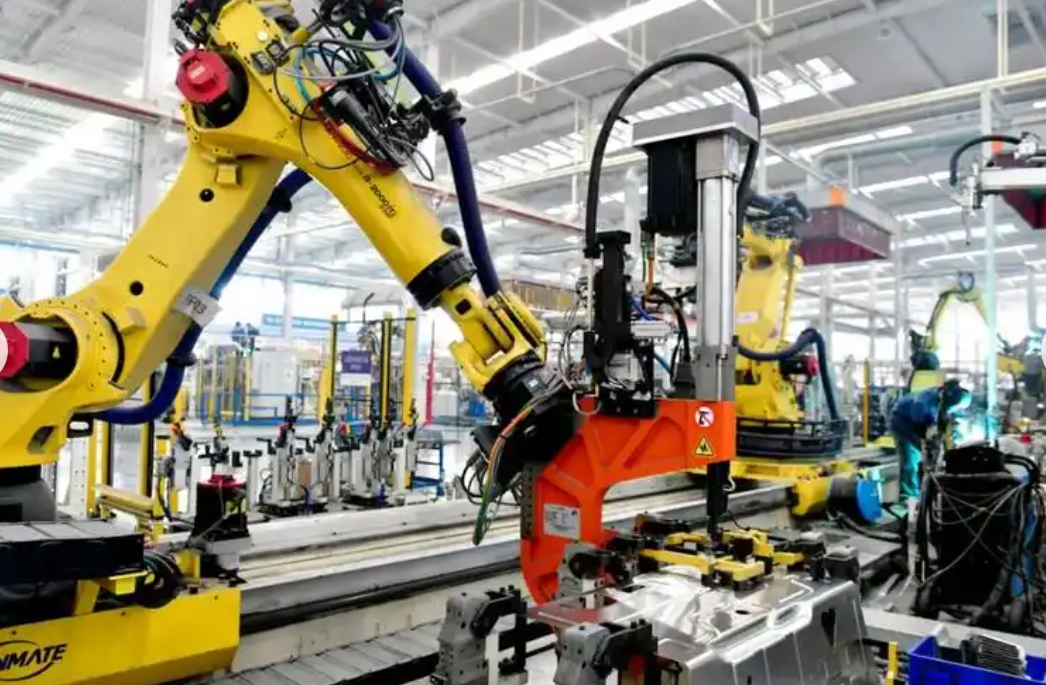
I model the robot as a six-degree-of-freedom serial chain. Joints 1, 2, and 3 primarily determine the position of the end effector, whereas joints 4, 5, and 6 primarily determine its orientation. Each joint is driven by a servo motor and a reducer, which provides smooth motion and high torque capacity. The kinematic behavior of industrial robots of this type is strongly influenced by the geometric relationship between adjacent joint axes. When adjacent joint axes are parallel, the conventional Denavit–Hartenberg (D-H) model suffers from parameter discontinuity and singularity. To overcome this limitation, I adopt the MD-H parameterization, which adds a rotation about the y-axis, denoted by \(\beta_i\), to the standard four D-H parameters \(\theta_i\), \(d_i\), \(a_i\), and \(\alpha_i\).
The MD-H parameter definitions used in my model are summarized in Table 1.
| Parameter | Definition | Type |
|---|---|---|
| \(\theta_i\) | Joint angle about the \(z_i\)-axis | Variable |
| \(d_i\) | Joint offset along the \(z_{i-1}\)-axis | Fixed |
| \(a_i\) | Link length along the \(x_i\)-axis | Fixed |
| \(\alpha_i\) | Link twist about the \(x_i\)-axis | Fixed |
| \(\beta_i\) | Rotation about the \(y_i\)-axis for parallel adjacent joints | Fixed |
Using the MD-H convention, the homogeneous transformation from frame \(\{i-1\}\) to frame \(\{i\}\) is expressed as
$$ {}^{i-1}T_i = R_z(\theta_i) T_z(d_i) T_x(a_i) R_x(\alpha_i) R_y(\beta_i) $$
where \(R_z\), \(R_x\), and \(R_y\) denote rotation matrices about the corresponding axes, and \(T_z\) and \(T_x\) denote translation matrices. The expanded form of the transformation matrix is
$$ {}^{i-1}T_i =
\begin{bmatrix}
c\theta_i c\beta_i – s\theta_i s\alpha_i s\beta_i & -s\theta_i c\alpha_i & -s\theta_i s\alpha_i c\beta_i + c\theta_i s\alpha_i & a_i c\theta_i \\
s\theta_i c\beta_i + c\theta_i s\alpha_i s\beta_i & c\theta_i c\alpha_i & c\theta_i s\alpha_i c\beta_i – s\theta_i s\alpha_i & a_i s\theta_i \\
-s\alpha_i c\beta_i & s\alpha_i & c\alpha_i & d_i \\
0 & 0 & 0 & 1
\end{bmatrix} $$
where \(s\) and \(c\) denote sine and cosine, respectively. The nominal MD-H parameters of the large-stroke heavy-load industrial robot are listed in Table 2. These values provide the starting point for forward kinematic computation and error modeling.
| Link \(i\) | Joint angle \(\theta_i\) (°) | Joint offset \(d_i\) (mm) | Link length \(a_i\) (mm) | Link twist \(\alpha_i\) (°) | Rotation \(\beta_i\) (°) |
|---|---|---|---|---|---|
| 1 | 0 | 675 | 350 | 0 | — |
| 2 | 0 | 0 | 1150 | −90 | 0 |
| 3 | −90 | 0 | 41 | 0 | — |
| 4 | 0 | 1200 | 0 | −90 | — |
| 5 | 0 | 0 | 0 | −90 | — |
| 6 | 180 | 215 | 0 | 0 | — |
The forward kinematic model of the industrial robot is obtained by multiplying the six link transformation matrices:
$$ {}^{0}T_6 = {}^{0}T_1 {}^{1}T_2 {}^{2}T_3 {}^{3}T_4 {}^{4}T_5 {}^{5}T_6 =
\begin{bmatrix}
n_x & o_x & a_x & p_x \\
n_y & o_y & a_y & p_y \\
n_z & o_z & a_z & p_z \\
0 & 0 & 0 & 1
\end{bmatrix} $$
where the vectors \(\mathbf{n}\), \(\mathbf{o}\), and \(\mathbf{a}\) describe the orientation of the end-effector frame, and \(\mathbf{p} = [p_x, p_y, p_z]^T\) describes its position. Since positioning accuracy is the primary concern for heavy-load industrial robots in high-precision operations, I focus on the position error rather than the orientation error. The position vector is a function of all kinematic parameters:
$$ \mathbf{p} = \mathbf{F}(\theta_1,\ldots,\theta_6, d_1,\ldots,d_6, a_1,\ldots,a_6, \alpha_1,\ldots,\alpha_6, \beta_2,\ldots,\beta_6) $$
In reality, the geometric parameters differ from their nominal values because of manufacturing and assembly errors. I therefore introduce the parameter error vector
$$ \Delta \mathbf{x} =
[\Delta \theta_1,\ldots,\Delta \theta_6,
\Delta d_1,\ldots,\Delta d_6,
\Delta a_1,\ldots,\Delta a_6,
\Delta \alpha_1,\ldots,\Delta \alpha_6,
\Delta \beta_2,\ldots,\Delta \beta_6]^T $$
The actual end-effector position can be written as
$$ \mathbf{p}’ = \mathbf{F}(\theta_i + \Delta \theta_i, d_i + \Delta d_i, a_i + \Delta a_i, \alpha_i + \Delta \alpha_i, \beta_i + \Delta \beta_i), \quad i = 1,\ldots,6 $$
By linearizing the forward kinematic model around the nominal parameters, the positioning error becomes
$$ \Delta \mathbf{p} = \mathbf{p}’ – \mathbf{p} \approx \mathbf{J} \Delta \mathbf{x} $$
where \(\mathbf{J}\) is the Jacobian matrix of the position vector with respect to the kinematic parameters. The Jacobian matrix is explicitly written as
$$ \mathbf{J} =
\begin{bmatrix}
\frac{\partial p_x}{\partial \theta_1} & \cdots & \frac{\partial p_x}{\partial \beta_6} \\
\frac{\partial p_y}{\partial \theta_1} & \cdots & \frac{\partial p_y}{\partial \beta_6} \\
\frac{\partial p_z}{\partial \theta_1} & \cdots & \frac{\partial p_z}{\partial \beta_6}
\end{bmatrix} $$
The geometric error sources that I consider are summarized in Table 3. These sources include link parameter errors, joint parameter errors, and the additional y-axis rotation terms required by the MD-H model. Since the industrial robot has a long reach and heavy payload, these errors are strongly coupled and can produce significant end-effector deviations.
| Error source | Symbol | Description | Influence on positioning |
|---|---|---|---|
| Joint angle error | \(\Delta \theta_i\) | Encoder offset and zero-position error | Large at base and shoulder joints |
| Joint offset error | \(\Delta d_i\) | Machining and assembly deviation along joint axis | Accumulates along kinematic chain |
| Link length error | \(\Delta a_i\) | Manufacturing error of link length | Directly scales with arm length |
| Link twist error | \(\Delta \alpha_i\) | Angular misalignment between adjacent axes | Produces coupled position and orientation error |
| Parallel-axis rotation error | \(\Delta \beta_i\) | Additional MD-H parameter for parallel joints | Removes singularity in D-H model |
To identify the parameter errors, I collect \(m\) sets of measured pose data, where \(m \ge 30\) ensures identifiability. For the \(j\)-th measurement, the measured position error is denoted by \(\delta \mathbf{x}_j\), and the corresponding Jacobian matrix is \(\mathbf{J}_j\). The conventional least-squares objective is
$$ \min_{\Delta \mathbf{x}} \sum_{j=1}^{m} \left\| \delta \mathbf{x}_j – \mathbf{J}_j \Delta \mathbf{x} \right\|^2 $$
The closed-form least-squares solution is
$$ \Delta \mathbf{x} = (\mathbf{J}^T \mathbf{J})^{-1} \mathbf{J}^T \delta \mathbf{x} $$
However, for large-stroke heavy-load industrial robots, the matrix \(\mathbf{J}^T \mathbf{J}\) is often ill-conditioned because of the large number of parameters and the strong coupling among them. This leads to slow convergence, unstable identification, and poor compensation accuracy. To address this issue, I use an improved iterative least-squares algorithm based on the Levenberg–Marquardt (L-M) method. The modified objective function is
$$ \min_{\Delta \mathbf{x}} \sum_{j=1}^{m} \left\| \delta \mathbf{x}_j – \mathbf{J}_j \Delta \mathbf{x} \right\|^2 + \lambda \left\| \Delta \mathbf{x} \right\|^2 $$
where \(\lambda\) is a damping factor. When \(\lambda\) is small, the algorithm behaves like the conventional least-squares method. When \(\lambda\) is large, the regularization term stabilizes the solution and prevents matrix singularity. The iterative update formula is
$$ \Delta \mathbf{x}_{k+1} = \Delta \mathbf{x}_k + (\mathbf{J}^T \mathbf{J} + \lambda \mathbf{I})^{-1} \mathbf{J}^T (\delta \mathbf{x} – \mathbf{J} \Delta \mathbf{x}_k) $$
where \(k\) is the iteration index and \(\mathbf{I}\) is the identity matrix. The identification process follows these steps: initialize the iteration count and the error vector, construct the linearized error equations, solve for the parameter increment using the damped least-squares formula, update the parameter estimate, and check whether the residual satisfies the preset accuracy threshold. If the threshold is not satisfied, I adjust the damping factor and repeat the iteration. When the residual converges, I output the identified parameter errors and write them into the robot controller for compensation.
The algorithm flow is summarized in Table 4.
| Step | Operation | Description |
|---|---|---|
| 1 | Initialize | Set \(k = 1\), \(\Delta \mathbf{x}_0 = 0\), and \(\lambda = \lambda_0\) |
| 2 | Construct error equations | Compute \(\delta \mathbf{x}_j\) and \(\mathbf{J}_j\) for all measured poses |
| 3 | Solve damped least-squares | Compute \(\Delta \mathbf{q} = (\mathbf{J}^T \mathbf{J} + \lambda \mathbf{I})^{-1} \mathbf{J}^T (\delta \mathbf{x} – \mathbf{J} \Delta \mathbf{x}_k)\) |
| 4 | Update parameters | \(\Delta \mathbf{x}_{k+1} = \Delta \mathbf{x}_k + \Delta \mathbf{q}\) |
| 5 | Check convergence | If residual is below threshold, stop; otherwise continue |
| 6 | Adjust damping | Reduce or increase \(\lambda\) according to residual behavior |
| 7 | Output | Return identified \(\Delta \mathbf{x}\) for compensation |
For the experimental validation, I build a calibration platform consisting of the large-stroke heavy-load industrial robot, a laser tracker, a spherically mounted retroreflector, and a host computer. The laser tracker has a measurement accuracy of \(\pm 0.01\) mm. The reflector is mounted on the end-effector flange. The robot is fixed on a vibration-isolated platform, and the laser tracker is placed 3–5 m away from the robot to ensure a stable line of sight. The host computer communicates with both the robot controller and the laser tracker for real-time data acquisition. The experimental devices and their functions are listed in Table 5.
| Device | Function | Key specification |
|---|---|---|
| Six-axis industrial robot | Motion and pose generation | Maximum reach 2700 mm, payload 210 kg |
| Laser tracker | End-effector position measurement | Accuracy \(\pm 0.01\) mm |
| Retroreflector | Measurement target | Installed on end-effector flange |
| Robot controller | Joint motion and compensation | Servo control and parameter update |
| Host computer | Data processing and identification | MATLAB-based computation |
Before calibration, I randomly select 50 points in the robot workspace. The robot is commanded to move to each point, and the laser tracker records the actual position while the controller records the joint angles. This first data set is used for parameter identification. After the error parameters are identified and compensated, the robot is commanded to move to the same 50 points again. The second data set is used to evaluate the improvement in positioning accuracy. The comparison between theoretical positions and measured positions before compensation is summarized in Table 6, where the values are reported as the mean absolute deviation over the selected points.
| Direction | Theoretical mean position (mm) | Measured mean position (mm) | Mean absolute deviation (mm) |
|---|---|---|---|
| \(x\) | — | — | 3.011 |
| \(y\) | — | — | 2.934 |
| \(z\) | — | — | 2.782 |
| Spatial | — | — | 5.778 |
After applying the improved iterative least-squares algorithm, I obtain the MD-H parameter errors listed in Table 7. These errors include joint angle offsets, joint offset deviations, link length deviations, link twist deviations, and the additional y-axis rotation terms. The identified values are then written into the controller as compensation parameters.
| Link \(i\) | \(\Delta \theta_i\) (°) | \(\Delta d_i\) (mm) | \(\Delta a_i\) (mm) | \(\Delta \alpha_i\) (°) | \(\Delta \beta_i\) (°) |
|---|---|---|---|---|---|
| 1 | 0 | 0.626 | 2.235 | 0 | — |
| 2 | 0 | 0.208 | −1.838 | 0.012 | 0 |
| 3 | −0.102 | 0.162 | −1.396 | 0.021 | — |
| 4 | −0.021 | 0.246 | 0.208 | 0.086 | — |
| 5 | −0.018 | 0.028 | 0.032 | 0.075 | — |
| 6 | 0.023 | 0.203 | −0.027 | 0.032 | — |
To quantify the compensation effect, I define the spatial comprehensive error as
$$ e = \sqrt{e_x^2 + e_y^2 + e_z^2} $$
where \(e_x\), \(e_y\), and \(e_z\) are the position errors along the three coordinate axes. I also compute the root mean square error (RMSE) as
$$ \text{RMSE} = \sqrt{\frac{1}{m} \sum_{j=1}^{m} e_j^2} $$
and the improvement ratio as
$$ \eta = \frac{E_{\text{before}} – E_{\text{after}}}{E_{\text{before}}} \times 100\% $$
The experimental results show that the proposed method substantially reduces the positioning error of the large-stroke heavy-load industrial robot. The maximum spatial error decreases from 19.257 mm to 1.278 mm, the mean spatial error decreases from 5.778 mm to 0.408 mm, and the spatial RMSE decreases from 6.949 mm to 0.481 mm. The detailed comparison is presented in Table 8.
| Error type | \(x\)-axis before (mm) | \(x\)-axis after (mm) | \(y\)-axis before (mm) | \(y\)-axis after (mm) | \(z\)-axis before (mm) | \(z\)-axis after (mm) | Spatial before (mm) | Spatial after (mm) |
|---|---|---|---|---|---|---|---|---|
| Maximum error | 15.105 | 0.613 | 11.907 | 0.769 | 9.611 | 1.276 | 19.257 | 1.278 |
| Mean error | 3.011 | 0.199 | 2.934 | 0.174 | 2.782 | 0.226 | 5.778 | 0.408 |
| RMSE | 4.293 | 0.246 | 3.969 | 0.236 | 3.757 | 0.340 | 6.949 | 0.481 |
The improvement percentages for each error index are summarized in Table 9. The maximum spatial error is reduced by 93.36%, the mean spatial error is reduced by 92.94%, and the spatial RMSE is reduced by 93.08%. Along the individual axes, the maximum error reductions are 95.94% in \(x\), 93.54% in \(y\), and 86.72% in \(z\). The mean error reductions are 93.39% in \(x\), 94.07% in \(y\), and 91.88% in \(z\). The RMSE reductions are 94.27% in \(x\), 94.05% in \(y\), and 90.95% in \(z\). These results confirm that the MD-H model combined with the improved iterative least-squares algorithm provides effective geometric error compensation for large-stroke heavy-load industrial robots.
| Index | \(x\)-axis improvement | \(y\)-axis improvement | \(z\)-axis improvement | Spatial improvement |
|---|---|---|---|---|
| Maximum error | 95.94% | 93.54% | 86.72% | 93.36% |
| Mean error | 93.39% | 94.07% | 91.88% | 92.94% |
| RMSE | 94.27% | 94.05% | 90.95% | 93.08% |
I further analyze the residual errors after compensation. The remaining error is mainly caused by non-geometric factors such as joint compliance, link deflection under heavy load, thermal drift, and measurement noise. Although the residual mean error is 0.408 mm, which is already suitable for many high-precision industrial applications, further improvement requires dynamic and non-geometric error modeling. For industrial robots with long strokes and heavy loads, the coupling between geometric and non-geometric errors is significant. Therefore, static geometric calibration should be regarded as the first stage of a broader accuracy enhancement framework.
The proposed calibration procedure can be repeated periodically to maintain accuracy. Because the identified parameters are stored in the controller, the compensation can be applied in real time during normal operation. The computational cost of the improved iterative least-squares algorithm is moderate, and the convergence is stable even when the Jacobian matrix is ill-conditioned. The damping factor \(\lambda\) plays a key role in balancing convergence speed and numerical stability. In my experiments, I start with a relatively large damping factor and reduce it gradually as the residual decreases. This strategy avoids large oscillations in the early iterations and achieves accurate parameter estimates in the later iterations.
The influence of the number of measurement points is also important. I use 50 points for identification and 50 points for validation. If the number of points is too small, the parameter identification may not be unique. If the number of points is too large, the measurement time increases and the influence of environmental drift becomes more pronounced. For large-stroke heavy-load industrial robots, the measurement points should cover the workspace as uniformly as possible, especially the regions where the arm is fully extended. In my experiments, the selected points cover both near and far reach configurations, which improves the observability of the kinematic parameters.
Table 10 summarizes the recommended calibration workflow for industrial robots of this class.
| Stage | Action | Purpose |
|---|---|---|
| Preparation | Fix robot and laser tracker, mount reflector, establish base frame | Ensure stable measurement conditions |
| Data collection | Move to 50 random points, record joint angles and measured positions | Provide identification data |
| Error modeling | Build MD-H model and linearized position error model | Relate parameter errors to end-effector error |
| Parameter identification | Apply improved iterative least-squares with damping | Estimate kinematic parameter errors |
| Compensation | Write identified errors into controller | Correct nominal kinematic parameters |
| Validation | Re-measure the same or new points | Evaluate accuracy improvement |
The experimental results demonstrate that the MD-H model is more suitable than the conventional D-H model for industrial robots with parallel adjacent joints. The additional \(\beta_i\) parameter removes the singularity that occurs when two consecutive joint axes are parallel. Without this parameter, the identification may become unstable and the compensation may be inaccurate. By including \(\beta_i\), I obtain a continuous and differentiable kinematic model that can represent the actual geometry of the industrial robot more faithfully. This is particularly important for large-stroke heavy-load industrial robots, because the long links amplify even small model discrepancies.
I also compare the convergence behavior of the conventional least-squares method and the improved iterative least-squares method. The conventional method often fails to converge when the Jacobian matrix is ill-conditioned. In contrast, the improved method converges smoothly because the damping term regularizes the normal equations. The residual decreases monotonically after a few iterations, and the identified parameters remain physically reasonable. This confirms that the improved algorithm is robust for multi-parameter coupling errors in large-stroke heavy-load industrial robots.
In terms of practical implementation, the proposed method has several advantages. First, it requires only a laser tracker and a reflector, which are common metrology tools in industrial environments. Second, the algorithm can be implemented in MATLAB or a similar numerical computing environment. Third, the compensation parameters can be integrated into the robot controller without changing the mechanical design. Fourth, the method is applicable to other industrial robots with similar structures, although the specific parameter values must be identified for each robot. These features make the method suitable for deployment in real production systems.
The remaining challenges include the following. Non-geometric errors such as joint compliance and link deflection are not fully captured by the static geometric model. Temperature variation can also cause gradual changes in the kinematic parameters. Future work should therefore incorporate online adaptation, multi-sensor fusion, and thermal error modeling. In addition, a more complete error model could include orientation errors and use full pose measurements. Although position accuracy is the main concern in many heavy-load tasks, orientation accuracy is also important in machining and assembly. I plan to extend the current framework to full pose calibration in future research.
In summary, I have presented a kinematic calibration and accuracy compensation method for large-stroke heavy-load industrial robots. The method is based on an MD-H kinematic model, a complete geometric error model, and an improved iterative least-squares identification algorithm. The experimental results show that the mean spatial positioning error is reduced from 5.778 mm to 0.408 mm, corresponding to an improvement of 92.94%. The maximum spatial error is reduced from 19.257 mm to 1.278 mm, and the spatial RMSE is reduced from 6.949 mm to 0.481 mm. These results indicate that the proposed method can significantly improve the absolute positioning accuracy of industrial robots and provide a practical solution for high-precision operations such as heavy assembly, precision inspection, and large-component machining.
For future work, I will focus on dynamic and thermal error compensation, online parameter updating, and full pose calibration. I will also investigate the integration of vision and force sensors to improve adaptability in complex environments. By combining geometric calibration with non-geometric compensation, it should be possible to achieve even higher accuracy and long-term stability for large-stroke heavy-load industrial robots. The proposed framework can serve as a foundation for developing intelligent calibration systems that automatically maintain accuracy throughout the lifecycle of industrial robots.