
In the field of robotics, the development of dexterous robotic hands has been a pivotal area of research, enabling machines to perform complex manipulation tasks that mimic human hand capabilities. As a researcher focused on robotic manipulation, I have dedicated significant effort to understanding and modeling the kinematics of such systems. Kinematics, which deals with the motion of bodies without considering the forces that cause them, is fundamental for controlling a dexterous robotic hand. Specifically, it allows us to describe the position, velocity, acceleration, and orientation of each joint and the end-effector, which is crucial for real-time control and precise manipulation. This article presents a comprehensive study on the kinematic model of a multi-fingered dexterous robotic hand, leveraging the Denavit-Hartenberg (DH) parameterization method. I will delve into the mechanical design, establish the DH model, derive both forward and inverse kinematics equations, and discuss their implications for control and planning. The goal is to provide a detailed foundation that can support advanced dynamics analysis, grasp planning, and motion control for dexterous robotic hands, ultimately enhancing their dynamic performance and optimal operational metrics.
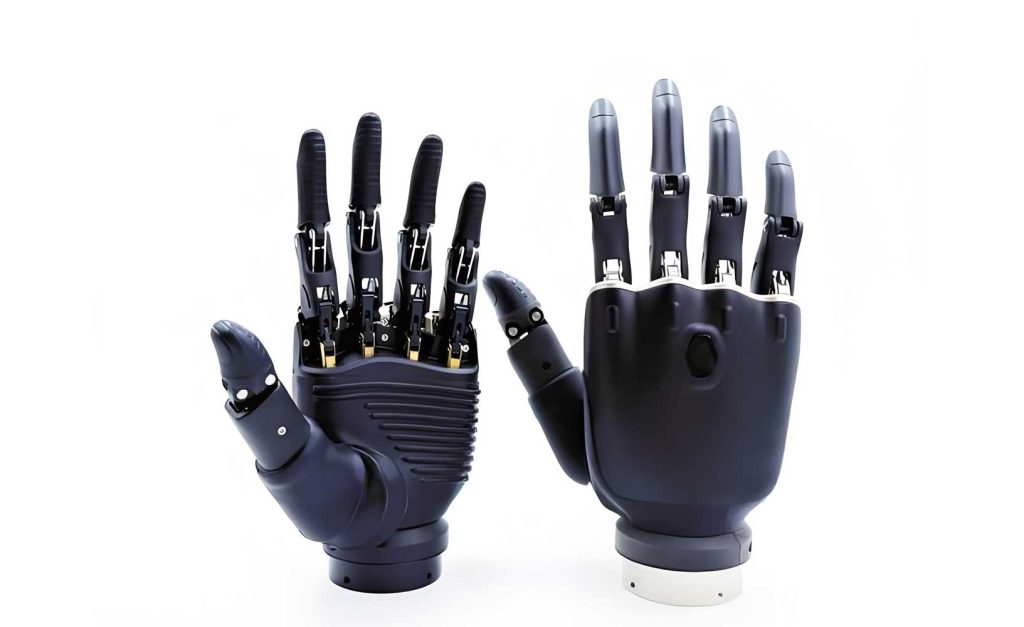
The mechanical structure of the dexterous robotic hand under consideration is inspired by human hand anatomy, designed to offer flexibility and adaptability in various grasping scenarios. This dexterous robotic hand consists of three identical fingers, each with three joints, a palm, and a wrist. Each finger includes a proximal phalanx, a medial phalanx, and a distal phalanx, corresponding to the human finger segments. The joints are revolute, allowing flexion and extension movements. To increase the versatility of this dexterous robotic hand, two of the fingers (referred to as F2 and F3) are capable of rotating within the palm plane over a range of 180 degrees, enabling adjustments for different object shapes and sizes. Additionally, the wrist is designed to rotate 360 degrees, further expanding the workspace and dexterity of the hand. The actuation mechanism involves micro DC motors for each joint, coupled with tendon-driven transmission, which provides compact and efficient force transmission. This design emphasizes lightweight construction and high precision, essential for a dexterous robotic hand intended for delicate tasks. The following table summarizes the key parameters of the finger joints:
| Joint Name | Length (mm) | Rotation Range (°) | Actuation Method | Transmission |
|---|---|---|---|---|
| Proximal Joint | 60 | 0–90 | Micro DC Motor | Tendon |
| Medial Joint | 40 | 0–90 | Micro DC Motor | Tendon |
| Distal Joint | 30 | 0–90 | Micro DC Motor | Tendon |
To analyze the motion of this dexterous robotic hand, we must establish a kinematic model that relates the joint variables to the position and orientation of the fingertip. The Denavit-Hartenberg (DH) convention is widely used for this purpose due to its systematic approach and clear physical interpretation. In this method, we attach a coordinate frame to each link of the robotic hand, starting from the base (palm) to the fingertip. The DH parameters—link length \(a_i\), link twist \(\alpha_i\), joint offset \(d_i\), and joint angle \(\theta_i\)—define the transformation between consecutive frames. For the dexterous robotic hand, since all joints are revolute, \(\theta_i\) is the variable of interest, while \(d_i\) is typically zero. The coordinate frames are assigned as follows: the \(z_i\)-axis aligns with the axis of joint \(i+1\), the \(x_i\)-axis is along the common perpendicular between \(z_i\) and \(z_{i-1}\), and the \(y_i\)-axis completes the right-handed coordinate system. This setup ensures consistency across all fingers, facilitating modular analysis. Below, I present the DH parameters for one finger (e.g., F1) of the dexterous robotic hand:
| Link \(i\) | \(\theta_i\) (Joint Variable) | \(\alpha_i\) (Link Twist) | \(d_i\) (Joint Offset) | \(a_i\) (Link Length) |
|---|---|---|---|---|
| 1 | \(\theta_1\) | 0° | 0 | \(l_1 = 60\) mm |
| 2 | \(\theta_2\) | 0° | 0 | \(l_2 = 40\) mm |
| 3 | \(\theta_3\) | 0° | 0 | \(l_3 = 30\) mm |
The homogeneous transformation matrix \(A_i\), which maps frame \(i\) to frame \(i-1\), is given by the standard DH formula:
$$ A_i = \begin{bmatrix} \cos\theta_i & -\sin\theta_i\cos\alpha_i & \sin\theta_i\sin\alpha_i & a_i\cos\theta_i \\ \sin\theta_i & \cos\theta_i\cos\alpha_i & -\cos\theta_i\sin\alpha_i & a_i\sin\theta_i \\ 0 & \sin\alpha_i & \cos\alpha_i & d_i \\ 0 & 0 & 0 & 1 \end{bmatrix} $$
For our dexterous robotic hand, since \(\alpha_i = 0\) and \(d_i = 0\), the matrix simplifies to:
$$ A_i = \begin{bmatrix} \cos\theta_i & -\sin\theta_i & 0 & a_i\cos\theta_i \\ \sin\theta_i & \cos\theta_i & 0 & a_i\sin\theta_i \\ 0 & 0 & 1 & 0 \\ 0 & 0 & 0 & 1 \end{bmatrix} $$
Substituting the values for each link, we obtain:
$$ A_1 = \begin{bmatrix} \cos\theta_1 & -\sin\theta_1 & 0 & l_1\cos\theta_1 \\ \sin\theta_1 & \cos\theta_1 & 0 & l_1\sin\theta_1 \\ 0 & 0 & 1 & 0 \\ 0 & 0 & 0 & 1 \end{bmatrix}, \quad A_2 = \begin{bmatrix} \cos\theta_2 & -\sin\theta_2 & 0 & l_2\cos\theta_2 \\ \sin\theta_2 & \cos\theta_2 & 0 & l_2\sin\theta_2 \\ 0 & 0 & 1 & 0 \\ 0 & 0 & 0 & 1 \end{bmatrix}, \quad A_3 = \begin{bmatrix} \cos\theta_3 & -\sin\theta_3 & 0 & l_3\cos\theta_3 \\ \sin\theta_3 & \cos\theta_3 & 0 & l_3\sin\theta_3 \\ 0 & 0 & 1 & 0 \\ 0 & 0 & 0 & 1 \end{bmatrix} $$
The forward kinematics of the dexterous robotic hand finger is then derived by multiplying these matrices in sequence, from the base to the fingertip. The overall transformation from the base frame to the fingertip frame (frame 3) is:
$$ {^0T_3} = A_1 A_2 A_3 = \begin{bmatrix} \cos(\theta_1 + \theta_2 + \theta_3) & -\sin(\theta_1 + \theta_2 + \theta_3) & 0 & l_1\cos\theta_1 + l_2\cos(\theta_1 + \theta_2) + l_3\cos(\theta_1 + \theta_2 + \theta_3) \\ \sin(\theta_1 + \theta_2 + \theta_3) & \cos(\theta_1 + \theta_2 + \theta_3) & 0 & l_1\sin\theta_1 + l_2\sin(\theta_1 + \theta_2) + l_3\sin(\theta_1 + \theta_2 + \theta_3) \\ 0 & 0 & 1 & 0 \\ 0 & 0 & 0 & 1 \end{bmatrix} $$
This matrix provides the position and orientation of the fingertip relative to the palm base. For convenience, let \(\phi_1 = \theta_1\), \(\phi_2 = \theta_1 + \theta_2\), and \(\phi_3 = \theta_1 + \theta_2 + \theta_3\). Then, the position coordinates \((x_p, y_p)\) of the fingertip in the base frame are:
$$ x_p = l_1\cos\phi_1 + l_2\cos\phi_2 + l_3\cos\phi_3 $$
$$ y_p = l_1\sin\phi_1 + l_2\sin\phi_2 + l_3\sin\phi_3 $$
These equations encapsulate the forward kinematics solution for a single finger of the dexterous robotic hand. They allow us to compute the fingertip location given the joint angles, which is essential for trajectory planning and control.
However, for fingers F2 and F3, which can rotate in the palm plane, an additional transformation is required to account for their base orientations. Specifically, the base frame for these fingers is offset and rotated relative to the palm coordinate system. Let \(\beta\) denote the fixed angle of the finger base relative to the palm (e.g., 0° for F1, and adjustable for F2 and F3), and \(\theta_0\) represent the rotational degree of freedom of the finger base (for F2 and F3, this can vary from 0 to 180°). The transformation from the palm frame to the finger base frame involves a translation along the x-axis by a distance \(l_0\) (the palm width offset), a rotation about the x-axis by \(\beta\), and a rotation about the z-axis by \(\theta_0\). The homogeneous transformation matrix \(A_0\) is:
$$ A_0 = \text{Rot}(z, \theta_0) \cdot \text{Rot}(x, \beta) \cdot \text{Trans}(l_0, 0, 0) $$
Where:
$$ \text{Rot}(z, \theta_0) = \begin{bmatrix} \cos\theta_0 & -\sin\theta_0 & 0 & 0 \\ \sin\theta_0 & \cos\theta_0 & 0 & 0 \\ 0 & 0 & 1 & 0 \\ 0 & 0 & 0 & 1 \end{bmatrix}, \quad \text{Rot}(x, \beta) = \begin{bmatrix} 1 & 0 & 0 & 0 \\ 0 & \cos\beta & -\sin\beta & 0 \\ 0 & \sin\beta & \cos\beta & 0 \\ 0 & 0 & 0 & 1 \end{bmatrix}, \quad \text{Trans}(l_0, 0, 0) = \begin{bmatrix} 1 & 0 & 0 & l_0 \\ 0 & 1 & 0 & 0 \\ 0 & 0 & 1 & 0 \\ 0 & 0 & 0 & 1 \end{bmatrix} $$
Thus, the complete forward kinematics for F2 and F3 fingers of the dexterous robotic hand is:
$$ {^0T_3} = A_0 A_1 A_2 A_3 $$
This extended model enables the dexterous robotic hand to adapt its finger placements for diverse grasping configurations, enhancing its manipulability.
While forward kinematics is straightforward, inverse kinematics is often more challenging but critical for control. Inverse kinematics involves determining the joint angles \((\theta_1, \theta_2, \theta_3)\) required to achieve a desired fingertip position \((x_p, y_p)\) and orientation \(\phi_3\). For the dexterous robotic hand, since the fingers operate primarily in a plane (ignoring the z-axis for simplicity), we can solve the inverse kinematics geometrically. Given the desired position \((x_p, y_p)\) and the final orientation angle \(\phi_3\), we define:
$$ r = \sqrt{x_p^2 + y_p^2}, \quad \alpha = \arctan\left(\frac{y_p}{x_p}\right) $$
From the geometry of the finger links, we have the vector loop equation:
$$ l_1 e^{i\phi_1} + l_2 e^{i\phi_2} + l_3 e^{i\phi_3} = r e^{i\alpha} $$
Where \(i\) is the imaginary unit. This complex equation represents the sum of link vectors in the plane. By separating real and imaginary parts, we obtain two scalar equations:
$$ l_1\cos\phi_1 + l_2\cos\phi_2 + l_3\cos\phi_3 = r\cos\alpha $$
$$ l_1\sin\phi_1 + l_2\sin\phi_2 + l_3\sin\phi_3 = r\sin\alpha $$
To solve for \(\phi_2\), we can eliminate \(\phi_1\). Rearranging terms and squaring both sides leads to:
$$ (r\cos\alpha – l_3\cos\phi_3)\cos\phi_2 + (r\sin\alpha – l_3\sin\phi_3)\sin\phi_2 = \frac{r^2 + l_2^2 + l_3^2 – l_1^2 – 2r l_3 \cos(\alpha – \phi_3)}{2l_2} $$
Let:
$$ A = r\cos\alpha – l_3\cos\phi_3, \quad B = r\sin\alpha – l_3\sin\phi_3, \quad C = \frac{r^2 + l_2^2 + l_3^2 – l_1^2 – 2r l_3 \cos(\alpha – \phi_3)}{2l_2} $$
Then, the equation becomes:
$$ A\cos\phi_2 + B\sin\phi_2 = C $$
This trigonometric equation can be solved using the tangent half-angle substitution, yielding two possible solutions for \(\phi_2\):
$$ \phi_2 = 2\arctan\left(\frac{B \pm \sqrt{B^2 + A^2 – C^2}}{A + C}\right) $$
Once \(\phi_2\) is known, \(\phi_1\) can be found from the original vector equations:
$$ \phi_1 = \arctan\left(\frac{r\sin\alpha – l_2\sin\phi_2 – l_3\sin\phi_3}{r\cos\alpha – l_2\cos\phi_2 – l_3\cos\phi_3}\right) $$
Finally, the joint angles are recovered using the relationships:
$$ \theta_1 = \phi_1, \quad \theta_2 = \phi_2 – \phi_1, \quad \theta_3 = \phi_3 – \phi_2 $$
Due to the mechanical constraints of the dexterous robotic hand (e.g., joint limits), we typically select the solution that is feasible and minimizes energy or path length. This inverse kinematics solution is vital for controlling the dexterous robotic hand to reach specific points in space, such as during object grasping or manipulation tasks.
To further elaborate on the kinematics of the dexterous robotic hand, let’s consider the velocity and acceleration analysis, which are derived from the Jacobian matrix. The Jacobian relates the joint velocities to the end-effector linear and angular velocities. For a planar finger, the Jacobian \(J\) can be computed from the position equations. Given \(x_p = l_1\cos\theta_1 + l_2\cos(\theta_1 + \theta_2) + l_3\cos(\theta_1 + \theta_2 + \theta_3)\) and \(y_p = l_1\sin\theta_1 + l_2\sin(\theta_1 + \theta_2) + l_3\sin(\theta_1 + \theta_2 + \theta_3)\), the Jacobian matrix is:
$$ J = \begin{bmatrix} \frac{\partial x_p}{\partial \theta_1} & \frac{\partial x_p}{\partial \theta_2} & \frac{\partial x_p}{\partial \theta_3} \\ \frac{\partial y_p}{\partial \theta_1} & \frac{\partial y_p}{\partial \theta_2} & \frac{\partial y_p}{\partial \theta_3} \end{bmatrix} $$
Computing these partial derivatives:
$$ \frac{\partial x_p}{\partial \theta_1} = -l_1\sin\theta_1 – l_2\sin(\theta_1 + \theta_2) – l_3\sin(\theta_1 + \theta_2 + \theta_3) $$
$$ \frac{\partial x_p}{\partial \theta_2} = -l_2\sin(\theta_1 + \theta_2) – l_3\sin(\theta_1 + \theta_2 + \theta_3) $$
$$ \frac{\partial x_p}{\partial \theta_3} = -l_3\sin(\theta_1 + \theta_2 + \theta_3) $$
$$ \frac{\partial y_p}{\partial \theta_1} = l_1\cos\theta_1 + l_2\cos(\theta_1 + \theta_2) + l_3\cos(\theta_1 + \theta_2 + \theta_3) $$
$$ \frac{\partial y_p}{\partial \theta_2} = l_2\cos(\theta_1 + \theta_2) + l_3\cos(\theta_1 + \theta_2 + \theta_3) $$
$$ \frac{\partial y_p}{\partial \theta_3} = l_3\cos(\theta_1 + \theta_2 + \theta_3) $$
Thus, the Jacobian is:
$$ J = \begin{bmatrix} -l_1\sin\theta_1 – l_2\sin(\theta_1 + \theta_2) – l_3\sin(\theta_1 + \theta_2 + \theta_3) & -l_2\sin(\theta_1 + \theta_2) – l_3\sin(\theta_1 + \theta_2 + \theta_3) & -l_3\sin(\theta_1 + \theta_2 + \theta_3) \\ l_1\cos\theta_1 + l_2\cos(\theta_1 + \theta_2) + l_3\cos(\theta_1 + \theta_2 + \theta_3) & l_2\cos(\theta_1 + \theta_2) + l_3\cos(\theta_1 + \theta_2 + \theta_3) & l_3\cos(\theta_1 + \theta_2 + \theta_3) \end{bmatrix} $$
Then, the end-effector velocity \(\dot{p} = [\dot{x}_p, \dot{y}_p]^T\) is related to joint velocities \(\dot{\theta} = [\dot{\theta}_1, \dot{\theta}_2, \dot{\theta}_3]^T\) by:
$$ \dot{p} = J \dot{\theta} $$
Similarly, acceleration can be derived by differentiating the velocity equation. This kinematic analysis is crucial for dynamic control and trajectory optimization of the dexterous robotic hand, ensuring smooth and accurate movements.
In addition to individual finger kinematics, the coordination of multiple fingers in the dexterous robotic hand is essential for complex grasping maneuvers. The overall hand kinematics involves combining the transformations of all fingers relative to a common palm frame. Let \(^0T_{3}^{(k)}\) denote the transformation for finger \(k\) (where \(k = 1, 2, 3\)). The palm frame is considered the base frame. For finger F1, the transformation is as derived earlier. For fingers F2 and F3, we incorporate the base rotation matrix \(A_0^{(k)}\) that depends on \(\theta_0^{(k)}\) and \(\beta^{(k)}\). The fingertip positions in the palm frame can then be used to compute grasp metrics such as the grasp matrix, which relates contact forces to net wrench on the object. This holistic approach enables the dexterous robotic hand to perform enveloping grasps, precision pinches, and other advanced manipulations.
To illustrate the application of the kinematic model, consider a scenario where the dexterous robotic hand needs to pick up a cylindrical object. Using inverse kinematics, we can compute the joint angles required to position the fingertips around the object’s circumference. Suppose the desired fingertip positions are given in the palm frame. For each finger, we solve the inverse kinematics equations to obtain \(\theta_1, \theta_2, \theta_3\). Then, through forward kinematics, we can verify the accuracy and adjust for collisions or singularities. The following table summarizes an example calculation for finger F1 with desired position \((x_p = 100\,\text{mm}, y_p = 50\,\text{mm})\) and orientation \(\phi_3 = 90^\circ\):
| Parameter | Value | Calculation |
|---|---|---|
| \(r\) | \(\sqrt{100^2 + 50^2} \approx 111.8\,\text{mm}\) | \(r = \sqrt{x_p^2 + y_p^2}\) |
| \(\alpha\) | \(\arctan(50/100) \approx 26.565^\circ\) | \(\alpha = \arctan(y_p/x_p)\) |
| \(A\) | \(100 – 30\cos(90^\circ) = 100\) | \(A = r\cos\alpha – l_3\cos\phi_3\) |
| \(B\) | \(50 – 30\sin(90^\circ) = 20\) | \(B = r\sin\alpha – l_3\sin\phi_3\) |
| \(C\) | \(\frac{111.8^2 + 40^2 + 30^2 – 60^2 – 2 \cdot 111.8 \cdot 30 \cos(26.565^\circ – 90^\circ)}{2 \cdot 40} \approx 1.5\) | \(C = \frac{r^2 + l_2^2 + l_3^2 – l_1^2 – 2r l_3 \cos(\alpha – \phi_3)}{2l_2}\) |
| \(\phi_2\) | \(2\arctan\left(\frac{20 + \sqrt{20^2 + 100^2 – 1.5^2}}{100 + 1.5}\right) \approx 53.13^\circ\) | Using positive root for feasibility |
| \(\phi_1\) | \(\arctan\left(\frac{50 – 40\sin(53.13^\circ) – 30\sin(90^\circ)}{100 – 40\cos(53.13^\circ) – 30\cos(90^\circ)}\right) \approx 18.43^\circ\) | \(\phi_1 = \arctan\left(\frac{r\sin\alpha – l_2\sin\phi_2 – l_3\sin\phi_3}{r\cos\alpha – l_2\cos\phi_2 – l_3\cos\phi_3}\right)\) |
| \(\theta_1\) | \(18.43^\circ\) | \(\theta_1 = \phi_1\) |
| \(\theta_2\) | \(53.13^\circ – 18.43^\circ = 34.70^\circ\) | \(\theta_2 = \phi_2 – \phi_1\) |
| \(\theta_3\) | \(90^\circ – 53.13^\circ = 36.87^\circ\) | \(\theta_3 = \phi_3 – \phi_2\) |
This example demonstrates the practical use of inverse kinematics for the dexterous robotic hand. It highlights how the model enables precise control of joint angles to achieve desired fingertip placements. Moreover, the forward kinematics can be used to validate the results by plugging \(\theta_1, \theta_2, \theta_3\) back into the forward equations, which should yield the original \((x_p, y_p)\) and \(\phi_3\).
Beyond basic kinematics, the dexterous robotic hand also involves considerations of singularities and workspace analysis. Singularities occur when the Jacobian matrix loses rank, leading to infinite joint velocities for some end-effector motions. For the planar finger, singularities happen when the links are fully extended or folded, causing the determinant of \(J\) to vanish. Analyzing these singularities helps in planning trajectories that avoid problematic configurations, ensuring stable control. The workspace of the dexterous robotic hand finger is the set of all points reachable by the fingertip. Given the link lengths and joint limits, the workspace is typically a region in the plane bounded by circles. For our finger with \(l_1=60\,\text{mm}, l_2=40\,\text{mm}, l_3=30\,\text{mm}\) and joint ranges of \(0^\circ\) to \(90^\circ\), the workspace can be computed numerically. The reachable points satisfy:
$$ \text{min reach} = \max(0, l_1 – l_2 – l_3) \quad \text{to} \quad \text{max reach} = l_1 + l_2 + l_3 $$
But due to joint limits, the actual workspace is a subset. Understanding the workspace is vital for grasp planning, as it defines the dexterous robotic hand’s ability to interact with objects of various sizes and positions.
Another important aspect is the integration of the kinematic model with control systems. For real-time operation of the dexterous robotic hand, we often use inverse kinematics solvers embedded in feedback loops. For instance, in position-based control, the desired fingertip trajectory is converted into joint angle commands via inverse kinematics, and encoders on the joints provide feedback for correction. Alternatively, velocity-based control uses the Jacobian to map desired end-effector velocities to joint velocities. The kinematic model derived here serves as the backbone for these control strategies. Moreover, for a multi-fingered dexterous robotic hand, coordination algorithms must synchronize the motions of all fingers to achieve stable grasps. This involves solving inverse kinematics for each finger while considering constraints like object geometry and contact points. Advanced techniques such as optimization-based inverse kinematics can handle redundancy (if present) and minimize effort or avoid obstacles.
In summary, this article has presented a detailed kinematic model for a dexterous robotic hand, focusing on the DH parameterization, forward kinematics, and inverse kinematics. The model provides a mathematical framework for analyzing and controlling the hand’s movements. The dexterous robotic hand’s design, with three fingers and adjustable bases, offers significant flexibility for manipulation tasks. The forward kinematics equations allow us to compute fingertip positions from joint angles, while the inverse kinematics solutions enable us to determine joint angles for desired positions. These foundations are essential for subsequent dynamics studies, grasp planning, and real-time control of the dexterous robotic hand. Future work may extend this model to include three-dimensional motions, contact forces, and compliance, further enhancing the capabilities of dexterous robotic hands in real-world applications such as manufacturing, healthcare, and service robotics.