
Dexterous robotic hand technology has found extensive applications in fields such as medical rehabilitation, intelligent robotics, and wearable devices. As a critical actuation unit for interaction between robots and the external environment, the performance of a dexterous robotic hand directly determines the flexibility and intelligence level of the robotic system. While traditional single-degree-of-freedom end-effectors are widely used in industrial scenarios due to their simplicity and ease of control, they exhibit limitations when handling complex object grasping tasks. Multi-degree-of-freedom dexterous robotic hands have thus become a vital research direction in robotics, aiming to achieve more precise manipulation and versatile grasping. Pneumatic artificial muscle (PAM)-driven dexterous robotic hands, known for their high safety, strong adaptability, and excellent power-to-weight ratio, have emerged as a key technology in this domain. Compared to electric motor and hydraulic drives, pneumatic muscles actuate flexible structures using compressed air, offering high contraction ratios and large output forces. This makes them suitable for compliant, lightweight designs and high-load scenarios. Although electric drives offer advantages in control precision, their output torque is limited by gearboxes and transmission structures, making it challenging to balance dexterous operation with grasp stability. Hydraulic drives, while providing strong load capacity, involve complex systems, large volumes, and high maintenance costs. Pneumatic muscles, combined with bio-inspired tendon structures and the compressibility of gas, can simulate the compliant deformation of biological muscles. Force transmission via tendons enables coordinated multi-degree-of-freedom motion, demonstrating superior environmental adaptability and safe force control.
In recent years, research on PAM-driven systems has garnered increasing attention. Scholars worldwide have proposed numerous advanced control methods to enhance system accuracy and stability. Traditional PID control, fuzzy control, and adaptive control have been widely applied to the modeling and control of PAM systems. For instance, fuzzy self-tuning PID control, position tracking controllers to improve joint angle tracking accuracy, and adaptive sliding mode controllers for enhanced trajectory tracking of robotic arms have been proposed. However, these methods still face limitations within PAM-driven systems, particularly concerning system nonlinearity, time-variance, and multi-joint coupling, failing to fully meet the demands for high precision and rapid response.
Model Predictive Control (MPC) has emerged as an effective control strategy, attracting widespread interest. MPC achieves optimal control for systems with multiple constraints through rolling-horizon optimization and feedback correction, making it particularly suitable for systems with significant dynamic variations and high coupling. Compared to traditional control methods, MPC demonstrates higher control precision and dynamic response capabilities for dexterous robotic hands under the nonlinear characteristics and multiple constraints inherent to PAM actuation. Mixed-integer predictive control and nonlinear MPC have been successfully implemented for trajectory tracking of spatial robotic arms. Despite its notable advantages, the traditional MPC framework relies on an accurate prediction model. The time-varying stiffness and nonlinear characteristics of PAM systems make model mismatch inevitable, limiting prediction accuracy and control performance.
To overcome this challenge, researchers have recently attempted to combine neural networks with MPC to form hybrid control methods. Backpropagation neural networks combined with MPC have been applied to robotic arms, hybrid controllers based on predictive control and iterative learning control have been proposed, and recurrent neural networks integrated with MPC have successfully addressed trajectory optimization for soft robotic hands. However, these methods still involve a trade-off between network structural complexity and real-time performance.
Given the limitations of existing research, this paper proposes a hybrid control method combining a Radial Basis Function (RBF) neural network with MPC. RBF neural networks, due to their local approximation properties and linear output weight distribution, are more suitable for the high-frequency control of pneumatic muscles. Successful applications of RBF-MPC architectures in autonomous vehicle trajectory tracking have been demonstrated. Therefore, building upon the RBF neural network and integrating it with the MPC optimization strategy, this paper proposes a novel controller aimed at addressing the nonlinearity, time-variance, and multi-joint coupling problems in PAM systems. Specifically, this paper first employs an RBF neural network to approximate the system’s nonlinear dynamic model; then derives a dynamic prediction model and designs the corresponding controller; finally, optimizes a cost function incorporating control input increments using the Newton-Raphson iterative algorithm to achieve high-precision trajectory tracking control for the PAM-driven dexterous robotic hand.
1. Modeling of the Three-Fingered Dexterous Robotic Hand
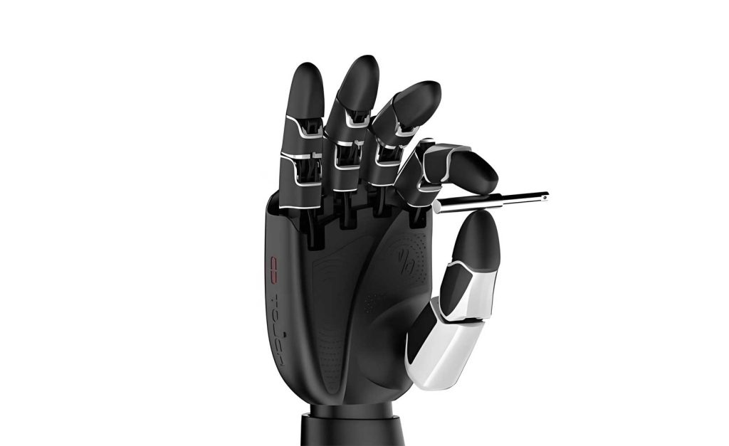
The designed three-fingered dexterous robotic hand comprises a PAM-driven assembly and three identically structured dexterous fingers. Each dexterous finger consists of three sequentially connected active finger joints, with pulley sets installed at each joint connection. Pneumatic muscles, controlled by pressure variations from an air source, contract and drive the pulley sets via tendons, causing the active finger joints to bend. This structure enables effective grasping and manipulation of various objects. The PAM-driven assembly includes the air source, pneumatic muscles, and tendons. The air source regulates pressure to control the contraction of the pneumatic muscles, which in turn pull the tendons to rotate the pulley sets, completing joint flexion. To enhance grasping force, angle sensors are mounted externally on the active joints of the dexterous fingers to monitor joint angle parameters in real-time. A fixed assembly, including sleeves, linear shafts, disks, and mounting brackets, ensures structural stability. This design provides higher control flexibility and precision.
1.1 Dynamic Experimental Modeling of the Dexterous Robotic Hand
To accurately obtain the angle information for each finger joint, angle sensors were installed at the three joints of each finger. Real-time acquisition of angle and pressure data is achieved through ADC sampling via serial communication between a computer and a microcontroller. By fitting the collected data, the mathematical relationship between the three joint angles was established, and the quantitative relationship between the angle and input pressure was further derived, with specific expressions as follows:
$$ \theta_1 + 0.749\theta_2 – 0.019\theta_3 – 1.563 = 0 $$
$$ \theta_1 = 1.3792u^2 – 142.5u + 28.96 $$
Here, $\theta_1$, $\theta_2$, $\theta_3$ represent the three joints of a single finger, and $u$ represents the input pressure to the pneumatic muscle.
1.2 RBF Neural Network Prediction Model
To accurately characterize the dynamic behavior of the PAM-driven dexterous robotic hand system, a nonlinear dynamic model is constructed directly. Due to the system’s inherently significant nonlinear characteristics, traditional linear modeling methods struggle to reflect the true system behavior, often leading to substantial modeling errors. Therefore, an RBF neural network with excellent nonlinear approximation capabilities is introduced for system modeling. The RBF network effectively establishes the dynamic relationship between input and output through nonlinear mapping, thereby modeling the system’s nonlinearity.
Although RBF neural networks offer significant advantages in nonlinear modeling, they have limitations in control applications: their structure lacks interpretability, making it difficult to customize control strategies accordingly; parameter settings heavily depend on prior knowledge, limiting adaptability. To overcome these issues, this paper introduces a linear dynamic modeling approach based on the RBF model, optimizing the model structure and key parameters to construct a nonlinear dynamic model that combines high modeling accuracy with good controllability:
$$
\begin{cases}
\mathbf{x}(k+1) = \mathbf{G}\mathbf{\Phi}(\mathbf{x}(k)) + \mathbf{H}u(k) + \mathbf{E}d(k) \\
y(k) = \mathbf{C}\mathbf{x}(k)
\end{cases}
$$
Where $\mathbf{x}(k) = [x_1(k), x_2(k)]^T$ is the state vector, $\mathbf{G} = [[g_{11}, g_{12}]; [g_{21}, g_{22}]]$ is the state coefficient matrix, $\mathbf{H} = [h_1; h_2]$ is the input coefficient matrix, $\mathbf{C} = [1, 0]$ is the output coefficient matrix, $\mathbf{E}(k) = [d_1; d_2]$ is the disturbance coefficient matrix, and $\mathbf{\Phi}(\mathbf{W}\mathbf{x}(k))$ is generated by the nonlinear mapping of the RBF network’s hidden layer, specifically:
$$ \Phi_j(\mathbf{x}(k)) = \exp\left(-\frac{||\mathbf{x}(k) – \mathbf{c}_j||^2}{2\sigma_j^2}\right) $$
Here, $\Phi_j(\mathbf{x}(k))$ denotes the $j$-th term of the radial basis function, $\mathbf{c}_j$ is the center of the $j$-th radial basis function, and $\sigma_j$ is its width.
2. Parameter Identification for the Nonlinear Dynamic Model
2.1 Parameter Identification Based on RBF Neural Network Algorithm
To construct the system’s nonlinear dynamic model, an RBF neural network is selected for parameter identification. In this process, we do not directly identify the RBF network’s own weights $\mathbf{W}$ or centers $\mathbf{c}_j$, but rather use the RBF neural network to model the system’s dynamic characteristics and optimize the model’s matrix parameters (e.g., $\mathbf{G}$, $\mathbf{H}$, $\mathbf{E}$). The goal is to enable the dynamic model to more accurately reflect the time-varying, nonlinear, and multi-joint coupling characteristics of the PAM-driven system. This choice is primarily based on the following considerations:
- RBF neural networks require a relatively small sample size for efficient modeling.
- Their simple structure, with only a single hidden layer, results in low computational overhead, ease of implementation, and helps prevent overfitting.
- They possess excellent nonlinear approximation capabilities, suitable for modeling systems with significant local nonlinear features.
Specifically, the RBF neural network establishes the relationship between input and output through nonlinear mapping. Then, parameter identification optimizes the model coefficients to improve accuracy and usability. The identification process includes two stages: forward propagation and parameter update. In forward propagation, the input signal is mapped to a high-dimensional space via radial basis functions, and the output layer generates the network output. The parameter update stage involves defining a loss function and iteratively optimizing network parameters using gradient descent to make the model output gradually approach the true value. This method effectively completes the parameter identification for the system’s dynamic model, with the specific procedure as follows:
1) Forward Propagation Stage
The output layer value of the RBF neural network can be expressed as:
$$ \mathbf{x}(k+1) = \mathbf{\Theta}^T \mathbf{\Psi}(\mathbf{x}(k), u(k), d(k)) $$
Where $\mathbf{\Theta} = [\mathbf{G}^T, \mathbf{H}^T, \mathbf{E}^T]^T$ is the parameter vector to be identified, and $\mathbf{\Psi}(\mathbf{x}(k), u(k), d(k)) = [\mathbf{\Phi}(\mathbf{x}(k))^T, u(k), d(k)]^T$ is the feature vector formed by mapping the input signal through radial basis functions.
The difference between the computed output of the nonlinear dynamic model and the desired output is defined as:
$$ \mathbf{e}(k) = \mathbf{x}(k) – \hat{\mathbf{x}}(k) $$
Here, $\mathbf{e}(k)$ represents the model’s state error vector, and $\hat{\mathbf{x}}(k)$ represents the model’s desired output vector.
The following objective function is chosen to measure the error:
$$ J(\mathbf{\Theta}) = \frac{1}{2} \sum_{k=1}^{M} ||\mathbf{e}(k)||^2 $$
Where $J(\mathbf{\Theta})$ is the objective function, and $M$ is the number of data samples.
2) Parameter Update Stage
Gradient descent is a typical method for solving optimization problems, used to adjust neural network parameters to minimize the objective function. Its basic update formula is:
$$ \mathbf{\Theta}(k+1) = \mathbf{\Theta}(k) – \eta \frac{\partial J}{\partial \mathbf{\Theta}} $$
Where $\mathbf{\Theta}(k)$ is the neural network parameter value at the current time step, $\mathbf{\Theta}(k+1)$ is the estimated value for the next time step, $\eta$ is the learning rate controlling the step size during parameter updates (typically in the range $(0,1)$), and $\frac{\partial J}{\partial \mathbf{\Theta}}$ is the gradient of the objective function with respect to parameters $\mathbf{\Theta}$, expressed as:
$$ \frac{\partial J}{\partial \mathbf{\Theta}} = -\sum_{k=1}^{M} \mathbf{\Psi}(\mathbf{x}(k), u(k), d(k)) \cdot \mathbf{e}(k+1) $$
Based on the gradient calculation formula, the parameters $\mathbf{G}$, $\mathbf{H}$, $\mathbf{E}$ can be updated separately:
$$ \mathbf{G}(k+1) = \mathbf{G}(k) – \eta \mathbf{e}(k) \mathbf{\Phi}(\mathbf{x}(k))^T + \alpha [\mathbf{G}(k) – \mathbf{G}(k-1)] $$
$$ \mathbf{H}(k+1) = \mathbf{H}(k) – \eta \mathbf{e}(k) u(k) + \alpha [\mathbf{H}(k) – \mathbf{H}(k-1)] $$
$$ \mathbf{E}(k+1) = \mathbf{E}(k) – \eta \mathbf{e}(k) d(k) + \alpha [\mathbf{E}(k) – \mathbf{E}(k-1)] $$
Here, $\alpha$ is the momentum factor, ranging from $[0,1]$, introduced to incorporate the cumulative effect of historical updates and prevent oscillations during parameter updates.
3) Objective Function and Parameter Determination
The learning rate $\eta$, momentum factor $\alpha$, and network iteration count $M$ for the RBF neural network are key parameters that need to be determined before identifying the nonlinear dynamic model parameters. The Mean Squared Error (MSE) can be used as the criterion for adjusting these three parameters. The MSE expression is:
$$ MSE = \frac{1}{N} \sum ||\mathbf{x}_t(k) – \mathbf{x}_p(k)||^2 $$
Where $N$ is the actual number of sample data points, $\mathbf{x}_t(k)$ is the actual sampled system data, and $\mathbf{x}_p(k)$ is the computed output data from the nonlinear dynamic model. By minimizing the MSE, the optimal hyperparameter configuration for the RBF neural network can be determined.
In this work, $\eta$, $\alpha$, and $M$ are treated as fixed prior training hyperparameters. Their values are obtained by minimizing the MSE on an independent validation set while simultaneously enforcing closed-loop realizability constraints (smooth control input increments, actuator non-saturation). Specifically, the learning rate $\eta$ is selected near the maximum stable value that ensures monotonic decrease of the loss function without oscillation. The momentum factor $\alpha$ is set to a moderate value that significantly accelerates convergence without inducing excessive oscillation. The iteration count $M$ is determined based on the “elbow” criterion of validation error decrease with increasing $M$, selecting the smallest $M$ when further increases yield diminishing returns.
2.2 Selection of Neural Network Internal Parameters
To determine the learning rate $\eta$, momentum factor $\alpha$, and required iteration count $M$ for the RBF neural network, a sinusoidal trajectory generated under PID control with a 0.01 s sampling frequency is used as identification data. This trajectory offers good continuity and variability, making it suitable as a reference input for system modeling and helpful for comprehensively evaluating the network’s identification performance.
(1) Selection of Learning Rate $\eta$
The learning rate $\eta$ determines the step size for network parameter updates, directly affecting training convergence speed and stability. A $\eta$ too small leads to slow convergence; too large may cause divergence. Therefore, with the momentum factor $\alpha$ fixed at 0, iteration counts $M$ of 1, 5, 10, and 50 are set, and identification comparisons are conducted under different $\eta$ values. Results show that as $\eta$ increases, the network achieves better MSE within a certain interval. Table 1 summarizes the MSE results under different combinations of learning rate and iteration count, used to define the reasonable range for the optimal learning rate.
| No. | Learning Rate $\eta$ | MSE (M=1) | MSE (M=5) | MSE (M=10) | MSE (M=50) |
|---|---|---|---|---|---|
| 1 | $10^{-8}$ | 2.729 | 3.330 | 1.157 | 1.600 |
| 2 | $10^{-7}$ | 2.154 | 0.628 | 1.075 | 1.322 |
| 3 | $10^{-6}$ | 1.273 | 2.759 | 1.416 | 1.186 |
| 4 | $10^{-5}$ | 3.356 | 1.728 | 0.953 | 0.776 |
| 5 | $10^{-4}$ | 1.520 | 2.338 | 2.339 | 2.704 |
| 6 | $10^{-3}$ | 1.664 | 1.260 | 2.106 | 2.322 |
| 7 | $10^{-2}$ | 0.966 | 0.541 | 1.923 | 1.725 |
| 8 | $10^{-1}$ | 1.461 | 0.900 | 0.728 | 0.089 |
From Table 1, it can be observed that when the learning rate is close to 0, the MSE is high. Even with an increased iteration count (M=50), the MSE remains elevated, indicating slow training progress as a learning rate too low is insufficient for network convergence. However, when the learning rate is close to 1, with fewer iterations (M=1), the MSE fluctuates significantly, even showing high errors, suggesting high learning rates can easily lead to instability. Therefore, assuming the network iteration count $M$ is 10, the learning rate $\eta$ can be selected from the interval $[10^{-8}, 10^{-7}, …, 10^{-2}]$.
(2) Determination of Momentum Factor $\alpha$
The momentum factor $\alpha$ can accelerate parameter convergence by incorporating historical gradients. However, an excessively large $\alpha$ may cause divergence. To balance convergence speed and stability, an incremental trial method is used to determine its optimal value. Selected momentum factors are 0.5, 0.9, and 0.99, corresponding roughly to assumptions of 2x, 10x, and 100x convergence acceleration, respectively. With the RBF neural network iteration count fixed at 10, the MSE values shown in Table 2 are obtained.
| No. | Learning Rate $\eta$ | MSE ($\alpha=0.5$) | MSE ($\alpha=0.9$) | MSE ($\alpha=0.99$) |
|---|---|---|---|---|
| 1 | $10^{-8}$ | 1.000 | 1.138 | 1.587 |
| 2 | $10^{-7}$ | 1.363 | 1.768 | 2.404 |
| 3 | $10^{-6}$ | 0.786 | 0.934 | 1.545 |
| 4 | $10^{-5}$ | 1.360 | 1.846 | 2.558 |
| 5 | $10^{-4}$ | 2.074 | 1.300 | 2.511 |
| 6 | $10^{-3}$ | 2.360 | 1.328 | 1.328 |
| 7 | $10^{-2}$ | 2.170 | 1.573 | 0.550 |
From Table 2, it can be seen that when the momentum factor is large (e.g., 0.99) combined with a low learning rate, it can easily lead to slow weight updates and increased error. Smaller momentum factors (e.g., 0.5 or 0.7) have less impact on the model and can stabilize the training process. Considering both convergence speed and accuracy, a momentum factor of 0.9 yields the best performance. Although the momentum factor is not the sole factor affecting accuracy, its proper setting can accelerate convergence and improve model performance.
The iteration count $M$ does not directly determine the network’s convergence accuracy or speed but significantly impacts training time. Increasing $M$ can reduce error to some extent but also increases computational cost. Therefore, a reasonable selection of $M$ helps ensure model performance while improving training efficiency. Based on the experimental results above, with learning rate $\eta = 10^{-2}$ and momentum factor $\alpha = 0.9$, initial values for the state coefficient matrix $\mathbf{G}$, input coefficient matrix $\mathbf{H}$, and disturbance coefficient matrix $\mathbf{E}$ are randomly generated, and five experiments are conducted to observe MSE changes under different iteration counts. The results are shown in Figure 2 (conceptual description). In all experiments, the MSE drops rapidly from a high initial value. After the iteration count reaches 10, the MSE for each experiment essentially converges. At this point, the model’s mean squared error stabilizes, indicating the RBF neural network training is complete.
In summary, the final selected neural network parameters are a learning rate $\eta$ of $10^{-2}$, a momentum factor $\alpha$ of 0.9, and an iteration count $M$ of 10.
3. Design of the RBF Model Predictive Controller
3.1 Nonlinear Prediction Model
The nonlinear dynamic model of the PAM-driven dexterous robotic hand is converted into state-space equation form, expressed as follows:
$$
\begin{cases}
\mathbf{x}(k+1|k) = \mathbf{G}\mathbf{\Phi}(\mathbf{x}(k|k)) + \mathbf{H}u(k|k) + \mathbf{E}d(k|k) \\
y(k+1|k) = \mathbf{C}\mathbf{x}(k+1|k)
\end{cases}
$$
Here, $\mathbf{x}(k+n|k)$ denotes the value predicted at time $(k+n)T$ based on $\mathbf{x}(k|k)$ at time $kT$. $\mathbf{x}(k|k) = [e(k|k); \dot{e}(k|k)]$ represents the state vector at time $kT$, where $e(k|k)$ is the error angle between the actual and predicted angles of the dexterous robotic hand’s finger, and $\dot{e}(k|k)$ is the error angular velocity. $\mathbf{x}(k+1|k) = [e(k+1|k); \dot{e}(k+1|k)]$ represents the state vector at time $(k+1)T$. $u(k|k)$ denotes the control law at time $kT$. $\mathbf{G} = [[g_{11}, g_{12}]; [g_{21}, g_{22}]]$ is the state coefficient matrix, $\mathbf{E} = [d_1; d_2]$ is the disturbance coefficient matrix, $\mathbf{H} = [h_1; h_2]$ is the input coefficient matrix, and $\mathbf{C} = [1, 0]$ is the output coefficient matrix. The nonlinear function $\mathbf{\Phi}(\mathbf{x}(k))$ is described by Equation (4). Therefore, the output $y(k+1|k)$ can be expressed as follows.
From Equation (14), the prediction model for time $(k+1)T$ can be formulated as:
$$ y(k+1|k) = \mathbf{C}\mathbf{G}\mathbf{\Phi}(\mathbf{x}(k|k)) + \mathbf{C}\mathbf{H}u(k|k) + \mathbf{C}\mathbf{E}d(k|k) $$
Based on the iterative nature of Equation (14), the nonlinear state-space equation at time $(k+2)T$ can be derived:
$$
\begin{cases}
\mathbf{x}(k+2|k) = \mathbf{G}\mathbf{\Phi}(\mathbf{x}(k+1|k)) + \mathbf{H}u(k+1|k) + \mathbf{E}d(k+1|k) \\
y(k+2|k) = \mathbf{C}\mathbf{x}(k+2|k)
\end{cases}
$$
From Equation (16), due to the nonlinearity of $\mathbf{\Phi}(\mathbf{x}(k))$, deriving the prediction model for subsequent time steps becomes difficult. To address the nonlinearity in the state-space equation, for future prediction time steps beyond $(k+1)T$, the nonlinear term in the prediction model is approximated as a linear term. The prediction model at time $(k+2)T$ can thus be derived as:
$$
\begin{aligned}
y(k+2|k) &= \mathbf{C}\mathbf{x}(k+2|k) \\
&= \mathbf{C}[\mathbf{G}\mathbf{\Phi}(\mathbf{x}(k+1|k)) + \mathbf{H}u(k+1|k) + \mathbf{E}d(k+1|k)] \\
&\approx \mathbf{C}[\mathbf{G}(\mathbf{K}\mathbf{x}(k+1|k) + \boldsymbol{\phi}) + \mathbf{H}u(k+1|k) + \mathbf{E}d(k+1|k)] \\
&= \mathbf{C}\mathbf{G}\mathbf{K}\mathbf{G}\mathbf{\Phi}(\mathbf{x}(k|k)) + \mathbf{C}\mathbf{G}\mathbf{K}\mathbf{H}u(k|k) + \mathbf{C}\mathbf{G}\mathbf{K}\mathbf{E}d(k|k) + \mathbf{C}\mathbf{G}\boldsymbol{\phi} \\
&\quad + \mathbf{C}\mathbf{H}u(k+1|k) + \mathbf{C}\mathbf{E}d(k+1|k)
\end{aligned}
$$
Therefore, through the prediction models shown in Equations (15) and (17), the prediction model for the dexterous robotic hand can be derived as:
$$ \mathbf{Y}(k) = \mathbf{G}(k)\mathbf{\Phi}(\mathbf{x}(k)) + \mathbf{H}(k)\mathbf{U}(k) + \mathbf{E}(k)\boldsymbol{\Delta}(k) $$
Here, $\mathbf{Y}(k)$ represents the system’s predicted angle error sequence, specifically:
$$ \mathbf{Y}(k) = [y(k+1|k)^T, y(k+2|k)^T, …, y(k+n|k)^T]^T = [e(k+1|k)^T, e(k+2|k)^T, …, e(k+n|k)^T]^T $$
$\mathbf{U}(k)$ represents the system’s control sequence:
$$ \mathbf{U}(k) = [u(k+1|k)^T, u(k+2|k)^T, …, u(k+m|k)^T]^T $$
$\boldsymbol{\Delta}(k)$ represents the system’s disturbance sequence:
$$ \boldsymbol{\Delta}(k) = [d(k+1|k)^T, d(k+2|k)^T, …, d(k+m|k)^T]^T $$
$\mathbf{H}(k)$ denotes the gain matrix of the prediction model, expressed in the form:
$$
\mathbf{H}(k) =
\begin{bmatrix}
\mathbf{C}\mathbf{H} & 0 & \cdots & 0 \\
\mathbf{C}\mathbf{G}\mathbf{K}\mathbf{H} & \mathbf{C}\mathbf{H} & \cdots & 0 \\
\vdots & \vdots & \ddots & \vdots \\
\sum_{i=0}^{n-1} \mathbf{C}(\mathbf{G}\mathbf{K})^{n-1-i}\mathbf{H} & \sum_{i=0}^{n-2} \mathbf{C}(\mathbf{G}\mathbf{K})^{n-2-i}\mathbf{H} & \cdots & \sum_{i=0}^{n-m} \mathbf{C}(\mathbf{G}\mathbf{K})^{n-m-i}\mathbf{H}
\end{bmatrix}
$$
$\mathbf{G}(k)$ and $\mathbf{E}(k)$ also represent gain matrices of the prediction model, with specific forms:
$$ \mathbf{G}(k) = [(\mathbf{C}\mathbf{G})^T, (\mathbf{C}\mathbf{G}\mathbf{K}\mathbf{G})^T, …, (\mathbf{C}(\mathbf{G}\mathbf{K})^{n-1}\mathbf{G})^T]^T $$
$$ \mathbf{E}(k) = [(\mathbf{C}\mathbf{E})^T, (\mathbf{C}(\mathbf{G}\mathbf{K})\mathbf{E})^T, …, (\mathbf{C}(\mathbf{G}\mathbf{K})^{n-1}\mathbf{E})^T]^T $$
Although the constructed prediction model is an approximate expression, the solved control law still maintains high accuracy. This is because MPC only employs the first control value in the current control sequence, and this value is determined by the predicted state at the current moment. According to Equation (15), the current predicted state can be accurately calculated. Since the prediction model on which this equation relies possesses high accuracy, the obtained control law can be considered reliable.
3.2 Cost Function for the RBF Neural Network Predictive Controller
For the established prediction model, assuming the predicted state $\mathbf{x}(k)$ at time $kT$ is known, and the predicted angle error sequence $\mathbf{Y}(k)$, gain matrices $\mathbf{G}(k)$, $\mathbf{H}(k)$, $\mathbf{E}(k)$, and nonlinear state variable $\mathbf{\Phi}(\mathbf{x}(k))$ contained in Equation (18) are also known, only the control sequence $\mathbf{U}(k)$ to be solved remains unknown in the system. To solve for the optimal control sequence $\mathbf{U}(k)$, MPC transforms the problem into a dynamic optimization problem. Therefore, a suitable cost function needs to be designed for the system. The cost function designed for the dexterous robotic hand is as follows:
$$ J = (\mathbf{Y} – \mathbf{Y}_{\text{ref}})^T \mathbf{Q}_1 (\mathbf{Y} – \mathbf{Y}_{\text{ref}}) + \mathbf{U}^T \mathbf{Q}_2 \mathbf{U} + \Delta\mathbf{U}^T \mathbf{Q}_3 \Delta\mathbf{U} $$
Here, $\mathbf{Y}$ is the system’s predicted output, and $\mathbf{Y}_{\text{ref}}$ is the system’s reference trajectory.
Taking the first-order difference between $J$ and $\mathbf{U}$ based on Equation (25) and expanding the solved first-order difference yields the following equation:
$$
\begin{aligned}
\frac{\partial J}{\partial \mathbf{U}} &= \frac{\partial}{\partial \mathbf{U}} \left[ (\mathbf{Y} – \mathbf{Y}_{\text{ref}})^T \mathbf{Q}_1 (\mathbf{Y} – \mathbf{Y}_{\text{ref}}) + \mathbf{U}^T \mathbf{Q}_2 \mathbf{U} + \Delta\mathbf{U}^T \mathbf{Q}_3 \Delta\mathbf{U} \right] \\
&= 2\mathbf{Q}_1 (\mathbf{Y} – \mathbf{Y}_{\text{ref}})^T \frac{\partial \mathbf{Y}}{\partial \mathbf{U}} + 2\mathbf{Q}_2 \mathbf{U} + 2\mathbf{Q}_3 \Delta\mathbf{U} \\
&= 2\mathbf{Q}_1 (\mathbf{Y} – \mathbf{Y}_{\text{ref}})^T \mathbf{H} + 2\mathbf{Q}_2 \mathbf{U} + 2\mathbf{Q}_3 \Delta\mathbf{U}
\end{aligned}
$$
The control Equation (26) is solved using the Newton-Raphson iterative algorithm to obtain the optimal control sequence $\mathbf{U}_k$. The first element of this control sequence is then applied to the system:
$$ u(k) = \mathbf{L} \mathbf{U}(k) $$
Where $\mathbf{L} = [1, 0, 0, …, 0]$.
4. Simulation and Experiment
4.1 Simulation and Analysis
To validate the effectiveness of the designed controller in terms of control accuracy, it is compared with MPC and T-S MPC, focusing on the angle tracking error of the first finger joint. The comparative MPC uses a nonlinear dynamic model as the prediction model and does not rely on RBF neural network parameter identification. Specifically, the prediction model is established based on the PAM pressure-contraction-mechanics relationship, tendon kinematics, and joint dynamics, with its structure and main parameters taken from the literature. Correspondingly, the T-S fuzzy rules, membership functions, and local linear sub-models for T-S MPC also follow the settings in the literature, maintaining consistent discretization and state definitions with traditional MPC. To ensure horizontal comparability, MPC, T-S MPC, and RBF MPC share identical parameters, with prediction horizon $n = 15$ and control horizon $m = 7$.
Simulation Validation of Angle Tracking Accuracy: To evaluate the tracking performance of RBF MPC, comparisons are made with MPC and T-S MPC under sinusoidal target curves with different amplitudes and periods. The simulation initial conditions are set to the same initial PAM pressure, and external disturbance $d(t) = \cos(0.4\pi t) – 0.4 \times \sin(0.1\pi t) \times e^{-0.2t}$ is introduced to simulate the actual operating environment. The tracking results are shown in Figure 3 (conceptual description). The results indicate that RBF MPC outperforms the comparison methods in angle tracking accuracy, validating the effectiveness of the proposed method.
Figure 3 (conceptual) shows the joint angle tracking performance of MPC, T-S MPC, and RBF MPC under different amplitudes and periods. From the simulation results, RBF MPC performs excellently in all tests, especially under larger amplitudes and higher frequencies, where its angle tracking accuracy is significantly better than MPC and T-S MPC. Regarding tracking error, RBF MPC exhibits the smallest error, with stability and precision far exceeding other methods. Therefore, RBF MPC shows clear advantages in joint angle tracking tasks for dynamic systems. The simulated data analysis results are recorded in Table 3.
| Control Algorithm | Related Data | (0.5 rad, 20 s) | (0.5 rad, 10 s) | (0.3 rad, 20 s) | (0.3 rad, 10 s) |
|---|---|---|---|---|---|
| MPC | Error Range [°] | [-0.046, 0.018] | [-0.085, 0.041] | [-0.030, 0.011] | [-0.053, 0.025] |
| MSE [°] | 0.0138 | 0.0289 | 0.0085 | 0.0176 | |
| MAE [°] | 0.0122 | 0.0257 | 0.0075 | 0.0155 | |
| T-S MPC | Error Range [°] | [-0.017, 0.015] | [-0.033, 0.033] | [-0.011, 0.009] | [-0.020, 0.020] |
| MSE [°] | 0.0114 | 0.0225 | 0.0070 | 0.0136 | |
| MAE [°] | 0.0103 | 0.0202 | 0.0063 | 0.0122 | |
| RBF MPC | Error Range [°] | [-0.016, 0.010] | [-0.031, 0.023] | [-0.010, 0.006] | [-0.019, 0.014] |
| MSE [°] | 0.0076 | 0.0157 | 0.0046 | 0.0095 | |
| MAE [°] | 0.0068 | 0.0141 | 0.0041 | 0.0085 |
From Table 3, it can be observed that when tracking different target curves under fixed disturbances, the maximum error, minimum error, MSE, and MAE of RBF MPC are all smaller than those of MPC and T-S MPC. This proves that the controller designed in this section has higher precision than the two comparative controllers for angle tracking of the dexterous robotic hand joint.
(2) Disturbance Rejection Capability Simulation of Control Algorithms: To verify the disturbance rejection capability of RBF MPC, ordinary MPC and T-S MPC are selected as comparative controllers, as in the previous simulation. A complex mixed curve is chosen as the reference target angle: $r(t) = 0.3 \times e^{\sin(0.3\pi t)} + 0.5 \times \cos(0.3\pi t)$. The initial PAM pressure is set to $p_0 = 2.5$ bar. By adding different external disturbances to the target curve, selected partial external disturbances are: Disturbance 1: $d_1(t) = 0.2 \times e^{\sin(0.1\pi t)} – 0.3 \times \cos(0.2\pi t)$; Disturbance 2: $d_2(t) = 0.5 \times \log(\sin(0.3\pi t) \times t + \cos(0.2\pi t))$. The simulation results are shown in Figure 4 (conceptual). From Figure 4, it can be seen that when tracking the same target curve under different disturbances, the error angle of RBF MPC is smaller than that of MPC and T-S MPC.
To more clearly demonstrate the disturbance rejection capability of RBF MPC, the simulation data above is analyzed and recorded in Table 4.
| Control Algorithm | Related Data | Disturbance 1 | Disturbance 2 |
|---|---|---|---|
| MPC | Error Range [°] | [-0.8077, 0.355] | [-0.8081, 0.3521] |
| MSE [°] | 0.0814 | 0.0847 | |
| MAE [°] | 0.0562 | 0.0591 | |
| T-S MPC | Error Range [°] | [-0.8028, 0.0775] | [-0.8028, 0.0825] |
| MSE [°] | 0.0501 | 0.0503 | |
| MAE [°] | 0.0384 | 0.0387 | |
| RBF MPC | Error Range [°] | [-0.8029, 0.3521] | [-0.8023, 0.2685] |
| MSE [°] | 0.0490 | 0.0490 | |
| MAE [°] | 0.0302 | 0.0305 |
Based on the comparative experimental results in Table 4, it can be concluded that under the same tracking target, whether subjected to sudden disturbances, instantaneous impact disturbances, or random fluctuation disturbances, RBF MPC significantly outperforms MPC and T-S MPC in terms of error fluctuation range, MSE, and MAE. This phenomenon fully verifies that the controller designed in this paper possesses superior disturbance suppression characteristics.
4.2 Experimental Platform Introduction
The pneumatically driven dexterous robotic hand employs an MPC closed-loop architecture. The host computer burns the program to an STM32F103 microcontroller, which generates analog voltage signals to drive proportional valves that regulate the output pressure from an air pump, thereby controlling the PAMs to drive the dexterous fingers. Angle sensors at the finger joints collect angle data in real-time and feed it back to the microcontroller, which then transmits the angle information to the host computer via serial communication, forming a closed loop for real-time tracking and dynamic optimization of the finger joint trajectory.
To meet the real-time requirements of the microcontroller platform, an offline-online division strategy is adopted: RBF neural network training and dynamic model parameter identification are performed offline on the host computer (determining the number of basis functions, centers $\mathbf{c}_j$, widths $\sigma_j$, weights $\mathbf{W}$, and generating the coefficient matrices required for the prediction model). The online stage on the STM32F103 performs lightweight computations only, including: lookup table/simple forward calculation for the offline-generated $\mathbf{\Phi}(\mathbf{x})$ and its Jacobian, a single linearization update using pre-computed prediction matrices, and execution of the Newton-Raphson iteration within a fixed number of steps, initialized with a warm start from the previous cycle’s solution. Under a unified control cycle setting, this online process can be stably completed within a single cycle, meeting real-time requirements. The baseline comparisons (traditional MPC, T-S MPC) also use the same sampling period, prediction/control horizons, and constraints, differing only in the source of the prediction model to ensure a fair comparison. The experimental process block diagram is shown in Figure 5 (conceptual).
To ensure comparability of results under different amplitude/frequency conditions, the experiments uniformly use a sampling period of 0.01 s. The three types of controllers (MPC, T-S MPC, RBF MPC) maintain the same prediction and control horizon parameters in the experiments (prediction horizon $n = 15$, control horizon $m = 7$). The proportional valves and PAMs start in the same stable initial state (identical initial pressure and pre-charge conditions), and joint initial angles are uniformly aligned (zero position calibration). The reference trajectories are four sets of sinusoidal curves with amplitudes of 0.5 rad and 0.3 rad, and periods of 10 s and 5 s, respectively.
4.3 Experimental Results and Analysis
Having validated the effectiveness and stability of the RBF neural network predictive controller through simulation, it is further verified on the dexterous robotic hand experimental platform. To evaluate the control performance of the proposed RBF MPC, comparative experiments are designed using sinusoidal signals with different periods and amplitudes as desired trajectories. The performance of RBF MPC is compared with T-S MPC and traditional MPC to further validate its effectiveness and superiority. The experimental results are shown in Figure 6 (conceptual).
After analyzing the experimental data, the results are recorded in Table 5.
| Control Algorithm | Related Data | (0.5 rad, 10 s) | (0.5 rad, 5 s) | (0.3 rad, 10 s) | (0.3 rad, 5 s) |
|---|---|---|---|---|---|
| MPC | Error Range [°] | [-3.483, 1.812] | [-2.867, 1.662] | [-6.128, 4.072] | [-3.518, 2.384] |
| MSE [°] | 1.2392 | 1.1437 | 2.6610 | 1.5904 | |
| MAE [°] | 1.1073 | 1.0234 | 2.3811 | 1.4262 | |
| T-S MPC | Error Range [°] | [-1.409, 1.424] | [-1.388, 1.404] | [-3.003, 3.041] | [-1.6615, 1.6821] |
| MSE [°] | 0.9347 | 0.9317 | 1.7788 | 1.0581 | |
| MAE [°] | 0.8410 | 0.8383 | 1.5973 | 0.9512 | |
| RBF MPC | Error Range [°] | [-1.430, 1.106] | [-1.256, 1.132] | [-2.422, 2.433] | [-1.312, 1.312] |
| MSE [°] | 0.7246 | 0.7469 | 1.3647 | 0.8068 | |
| MAE [°] | 0.6501 | 0.6715 | 1.2219 | 0.7247 |
Analysis of the data in the table leads to the following conclusions: As the reference trajectory frequency increases from a 10 s period to a 5 s period, the error metrics (error range, MSE, MAE) for all three controllers increase to varying degrees, reflecting the effective bandwidth and charge/discharge time lag limitations of the PAM-valve system. Under the same conditions, the increase in metrics for RBF MPC is smaller, indicating its stronger compensation capability for frequency domain gain and phase lag. In the 0.3 rad condition compared to 0.5 rad, joint angular velocity and pressure difference swing decrease, and the signal-to-noise ratio drops, making MAE/MSE more sensitive to measurement noise. RBF MPC still maintains error levels superior to MPC and T-S MPC, demonstrating better adaptability to nonlinearities and friction dead zones in small-signal regions.
Across the four amplitude-frequency combinations, RBF MPC achieves the smallest error range, MSE, and MAE, and is less sensitive to the adverse effects caused by increased frequency and decreased amplitude, exhibiting superior tracking stability and robustness.
To further validate the effectiveness of the proposed algorithm, the reference angle trajectory is extended from a sinusoidal signal to other types of input signals (e.g., $r(t) = 0.4 \times e^{\sin(0.4\pi t)}$), and the performance of the proposed controller is compared and analyzed against other controllers on this basis to comprehensively evaluate its robustness and adaptability. The experimental results are shown in Figure 7 (conceptual).
After analyzing the above experimental results, the relevant data is summarized in Table 6.
| Control Algorithm | Error Range [°] | MSE [°] | MAE [°] |
|---|---|---|---|
| MPC | [-23.2704, 7.5615] | 1.8616 | 1.1538 |
| T-S MPC | [-23.0556, 5.8681] | 1.2537 | 0.8186 |
| RBF MPC | [-23.0456, 1.6011] | 1.1623 | 0.7138 |
From the data in the table, it can be seen that the controller designed in this paper exhibits superior tracking performance when following complex reference signals, offering better control accuracy and stability compared to the benchmark controllers.
The experimental results indicate that RBF MPC holds significant advantages over the two baseline methods (MPC, T-S MPC), primarily manifested in:
- RBF identification improves the prediction model’s fit to the PAM’s time-varying/nonlinear characteristics, reducing rolling optimization bias caused by model mismatch.
- The cost function explicitly includes a $\Delta u$ term, suppressing rapid opening/closing of proportional valves and severe fluctuations in chamber pressure differences, thereby reducing overshoot and steady-state oscillation.
- The use of the Newton-Raphson iterative algorithm to solve the incremental control law enables faster convergence of online optimization within the same sampling period, reducing phase lag in high-frequency conditions.
5. Conclusion
This paper proposed a hybrid control method combining a Radial Basis Function neural network with Model Predictive Control to enhance the trajectory tracking accuracy of a pneumatic muscle-driven dexterous robotic hand. Through simulation and experimental validation, the results demonstrated that under sinusoidal target curves with different amplitudes and periods, the angle tracking error of RBF MPC was significantly smaller than that of traditional MPC and T-S MPC controllers. Particularly under conditions of larger amplitude and higher frequency, RBF MPC exhibited notable precision advantages, reflected in its lower mean squared error and mean absolute error compared to the other two controllers, indicating higher control precision and robustness.
Experimental results showed that under dynamic variations and external disturbances, RBF MPC maintained a low error range, proving its strong disturbance rejection capability. Especially in scenarios of frequency change and amplitude reduction, the increase in error for RBF MPC was smaller, demonstrating stronger adaptability, particularly to nonlinear characteristics and decreased signal-to-noise ratio.
Although RBF MPC demonstrated superior performance in this study, some limitations remain. First, the current research primarily focused on standard sinusoidal trajectories and disturbances, without considering more complex nonlinear input signals and complex disturbances in practical application scenarios. Second, the training process of the RBF neural network relies on data quality and quantity. Future work could improve the model’s generalization ability and real-time performance by optimizing training strategies and network structures.
This research provides an effective approach for further optimizing the control performance of PAM-driven systems. Future studies could proceed in the following directions: Firstly, investigate extension methods for RBF MPC by incorporating more types of nonlinear dynamics and complex environmental disturbances to enhance its performance in complex tasks. Secondly, promote the application of the RBF MPC controller on actual hardware platforms, optimizing real-time performance and computational resource constraints to improve online control efficiency. Finally, explore the application of RBF MPC in multi-degree-of-freedom dexterous hand manipulation and multi-object cooperative grasping tasks to further enhance its control capability in complex dynamic environments.