
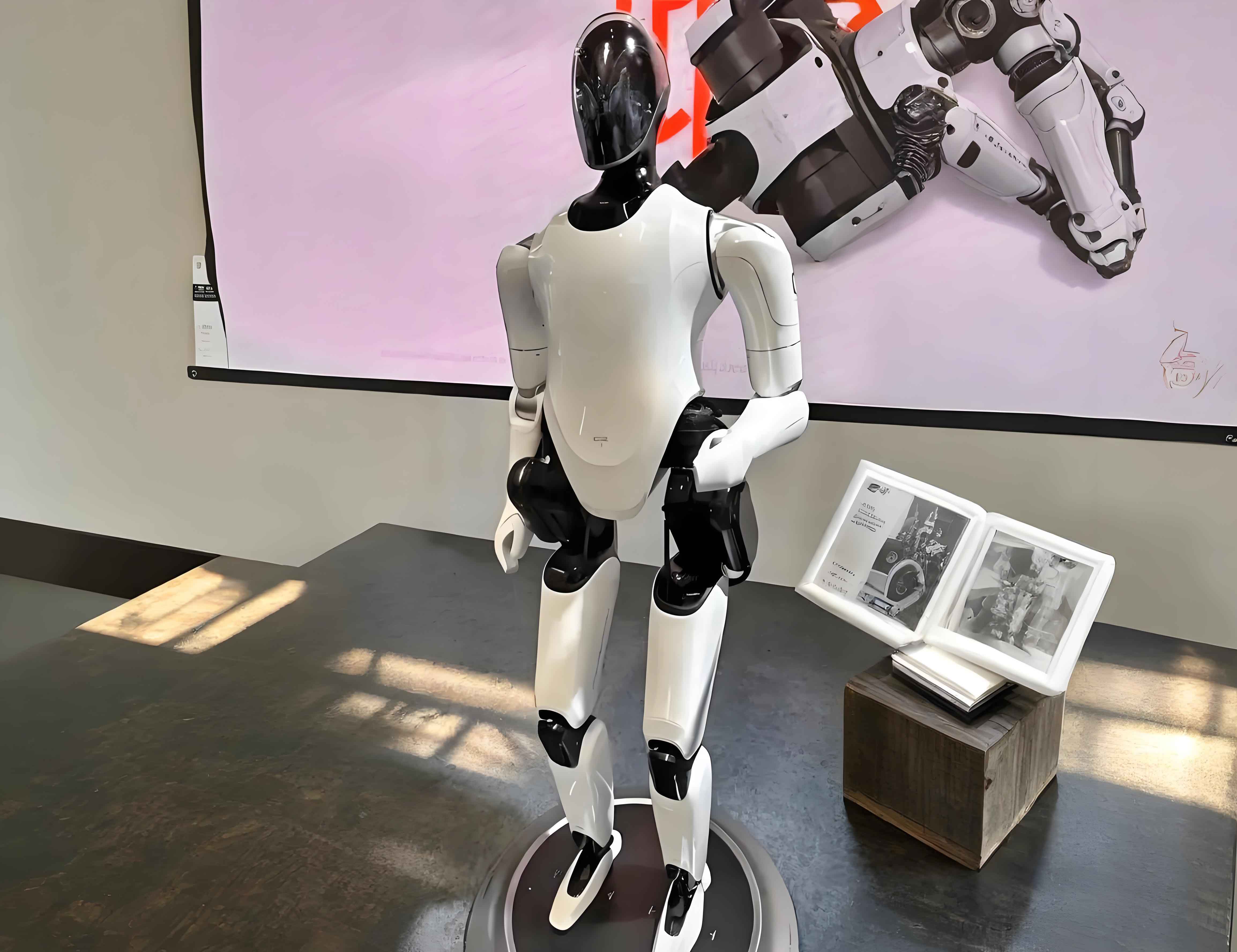
Humanoid robotics has evolved into one of the most active research frontiers in modern engineering. The unique value of a humanoid robot lies in its ability to move through environments designed for humans, using bipedal locomotion as the fundamental mode of transport. Such a machine is a quintessential embodiment of the concept of an embodied robot, where intelligence and motor behavior are tightly coupled through physical form, sensing, and actuation. This thesis focuses on the motion control of an embodied robot built on the NAO humanoid platform, with the central goal of achieving stable, efficient, and natural walking. The work encompasses kinematic modeling, parameterized gait planning, multi-objective optimization, and virtual prototyping simulation. By studying the NAO robot as a representative embodied robot, the findings provide practical insights into bipedal locomotion and control that can be extended to other humanoid systems.
The study of humanoid walking is not only scientifically challenging but also technologically relevant. The humanoid form enables a machine to operate in cooperation with humans in domestic, medical, and industrial settings. Compared with wheeled mobile robots, an embodied robot with two legs can step over obstacles, climb stairs, and adapt to irregular terrain. However, these capabilities come at the cost of complex dynamics, high-dimensional actuation, and stringent stability requirements. In particular, the walking process involves alternating between single-support and double-support phases, which forces the controller to continuously balance gravitational and inertial effects. Therefore, gait planning and motion control are the core issues in deploying an embodied robot in real-world environments.
This paper presents a systematic investigation of the NAO humanoid robot, which is 58 cm tall, weighs approximately 4.5 kg, and possesses 25 degrees of freedom. The lower body contains eleven degrees of freedom, including hip, knee, and ankle joints. The detailed joint arrangement allows the embodied robot to generate versatile walking motions. To formulate a tractable control strategy, I first establish a complete kinematic model using the Denavit–Hartenberg convention. Next, I design a parametric gait for straight-line walking based on the zero-moment-point stability criterion. The gait is generated through polynomial interpolation of the ankle and hip trajectories, followed by inverse kinematics to obtain joint angle profiles. I then optimize the gait parameters using a genetic algorithm, simultaneously considering walking stability, energy consumption, and speed. Finally, I build a virtual prototype in ADAMS and verify the planned gait through dynamic simulation. The simulation results confirm that the optimized embodied robot can perform stable and smooth bipedal walking.
1 Kinematic Modeling of the Embodied Robot
Kinematics is the foundation for robot motion planning and control. For an embodied robot, the kinematic model maps joint angles to link positions and orientations, and vice versa. In this section, I describe the NAO robot lower-limb structure and derive the forward and inverse kinematic equations using the Denavit–Hartenberg (D-H) parameterization.
1.1 Robot Description and Coordinate Frames
The NAO robot lower body includes two legs, each with five revolute joints: two at the hip (roll and pitch), one at the knee (pitch), and two at the ankle (pitch and roll). The hip yaw joint is shared between the two legs through a differential mechanism, giving a total of five actuators per leg. This arrangement is sufficient for walking in the sagittal and frontal planes. Table 1 lists the mass and length parameters of the lower-body links.
| Link | Joint | Mass (g) | Length (mm) | DOF |
|---|---|---|---|---|
| Torso | — | 2967.12 | 211.5 | 1 |
| Thigh | Hip | 520.25 × 2 | 100 | 3 × 2 |
| Shank | Knee | 291.525 × 2 | 102.9 | 1 × 2 |
| Ankle | Ankle | 134.15 × 2 | — | 2 × 2 |
| Foot | — | 164.77 × 2 | 45.19 | — |
Each joint is bounded by mechanical limits. The motion ranges for the left and right legs are given in Table 2. These constraints are essential for ensuring that the planned trajectories remain physically feasible.
| Joint | Range (deg) | Range (rad) |
|---|---|---|
| Hip yaw | -65.62 to 42.44 | -1.145303 to 0.740810 |
| Hip roll | -21.74 to 45.29 | -0.379472 to 0.790477 |
| Hip pitch | -101.54 to 27.82 | -1.772308 to 0.485624 |
| Knee pitch | -5.90 to 121.47 | -0.103083 to 2.120198 |
| Ankle pitch | -68.15 to 52.86 | -1.189516 to 0.922747 |
| Ankle roll | -22.27 to 45.03 | -0.388676 to 0.785875 |
To build the kinematic model, I place local coordinate frames at each joint following the D-H convention. The transformation between consecutive frames \(i-1\) and \(i\) is represented by the homogeneous matrix
$$T_i^{i-1} = \begin{bmatrix}
\cos\theta_i & -\sin\theta_i \cos\alpha_i & \sin\theta_i \sin\alpha_i & a_i \cos\theta_i\\
\sin\theta_i & \cos\theta_i \cos\alpha_i & -\cos\theta_i \sin\alpha_i & a_i \sin\theta_i\\
0 & \sin\alpha_i & \cos\alpha_i & d_i\\
0 & 0 & 0 & 1
\end{bmatrix},$$
where \(a_i\) is the link length, \(\alpha_i\) is the link twist, \(d_i\) is the link offset, and \(\theta_i\) is the joint angle. For the lower-limb model of the embodied robot, the D-H parameters are summarized in Table 3.
| Link \(i\) | \(\alpha_{i-1}\) (rad) | \(a_{i-1}\) (mm) | \(\theta_i\) (rad) | \(d_i\) (mm) |
|---|---|---|---|---|
| 1 | 0 | 0 | \(\theta_1\) | 0 |
| 2 | \(\pi/2\) | 0 | \(\theta_2\) | 0 |
| 3 | 0 | 102.9 | \(\theta_3\) | 0 |
| 4 | 0 | 100 | \(\theta_4\) | 0 |
| 5 | \(-\pi/2\) | 0 | \(\theta_5\) | 0 |
| 6 | \(-\pi/2\) | 0 | \(\theta_6\) | 0 |
| 7 | \(\pi\) | 50 | \(\theta_7\) | 0 |
| 8 | \(-\pi/2\) | 0 | \(\theta_8\) | 0 |
| 9 | \(-\pi/2\) | 0 | \(\theta_9\) | 0 |
| 10 | 0 | 100 | \(\theta_{10}\) | 0 |
| 11 | 0 | 102.9 | \(\theta_{11}\) | 0 |
| 12 | \(\pi/2\) | 0 | \(\theta_{12}\) | 0 |
1.2 Forward Kinematics
Forward kinematics computes the pose of the foot relative to the hip from the joint angles. By multiplying the individual D-H matrices according to the chain rule, the overall transformation from frame 6 to frame 0 is
$$T_6^0 = T_1^0 T_2^1 T_3^2 T_4^3 T_5^4 T_6^5.$$
After applying the D-H parameters, the resulting forward kinematic equation can be written in the form
$$T_6^0 = \begin{bmatrix}
N_x & O_x & A_x & P_x\\
N_y & O_y & A_y & P_y\\
N_z & O_z & A_z & P_z\\
0 & 0 & 0 & 1
\end{bmatrix},$$
with the following entries:
$$N_x = C_{11} C_{2+3+4} C_{5+6} + S_{11} S_{5+6},$$
$$O_x = -C_{11} C_{2+3+4} S_{5+6} + S_{11} C_{5+6},$$
$$A_x = -C_{11} S_{2+3+4},$$
$$P_x = C_{11} (C_{2+3} \cdot 102.9 + C_2 \cdot 100),$$
$$N_y = -S_{11} C_{2+3+4} C_{5+6} + C_{11} S_{5+6},$$
$$O_y = S_{11} C_{2+3+4} S_{5+6} + C_{11} C_{5+6},$$
$$A_y = -S_{11} S_{2+3+4},$$
$$P_y = -S_{11} (C_{2+3} \cdot 102.9 + C_2 \cdot 100),$$
$$N_z = -S_{2+3+4} C_{5+6},$$
$$O_z = S_{2+3+4} S_{5+6},$$
$$A_z = -C_{2+3+4},$$
$$P_z = -(S_{2+3} \cdot 102.9 + S_2 \cdot 100).$$
Here, the shorthand notation \(C_{2+3+4}\) denotes \(\cos(\theta_2+\theta_3+\theta_4)\), and similarly for the sine functions. The forward kinematics is useful for verifying trajectories and computing Jacobian-based quantities.
1.3 Inverse Kinematics
For gait planning, the inverse kinematics problem must be solved: given the desired hip and ankle positions, calculate the joint angles of the leg. The lower limb of the embodied robot can be represented as a two-link leg from the hip to the ankle, with the knee angle determined by the distance between the hip and ankle. Let \(\mathbf{P} = [P_x, P_y, P_z]^T\) be the ankle position relative to the hip, and let \(l_t = 100\) mm be the thigh length, \(l_s = 102.9\) mm be the shank length, and \(l_b = |\mathbf{P}|\). Then the knee angle is
$$\theta_3 = \pi – \arccos\!\left(\frac{l_t^2 + l_s^2 – l_b^2}{2 l_t l_s}\right).$$
The hip yaw angle is
$$\theta_1 = \operatorname{atan2}(P_y, P_x).$$
The hip pitch angle is
$$\theta_2 = -\alpha + \operatorname{atan2}\!\left(P_z, \operatorname{sign}(P_x)\sqrt{P_x^2 + P_y^2}\right),$$
where \(\alpha\) is the angle at the ankle side of the triangle formed by the thigh, shank, and the line from hip to ankle:
$$\alpha = \arcsin\!\left(\frac{l_s \sin(\pi – \theta_3)}{l_b}\right).$$
The ankle pitch is then
$$\theta_4 = \theta_2 – \theta_3,$$
and the ankle roll and hip roll are determined by the lateral displacement. The remaining angles are obtained by solving the orientation part of the transformation matrix. Because the lower limb of the embodied robot is symmetric, the same equations apply to both legs with appropriate sign changes.
2 Parameterized Gait Trajectory Design
Gait planning determines the time evolution of all joint angles so that the robot moves according to prescribed step length, step height, and walking speed. For the NAO robot, I adopt a parallel gait pattern in which the torso stays upright and the feet remain parallel to the ground. This simplifies the planning because the torso orientation is fixed and only the lower-limb trajectories need to be designed. A stable walking gait is generated using the three-step planning method:
- Step 1: Plan the foot and hip trajectories based on the walking phase, using polynomial interpolation.
- Step 2: Derive all other joint angles from the inverse kinematics equations.
- Step 3: Refine the trajectories to ensure smoothness and repeatability.
2.1 Stability Criterion Based on ZMP
The zero-moment point (ZMP) is widely used as the stability criterion for legged robots. The ZMP is defined as the point on the ground where the resultant ground reaction force acts. For a statically and dynamically stable walk, the ZMP must lie strictly inside the support polygon formed by the foot or feet in contact with the ground. The ZMP of a multi-body system can be computed as
$$x_{\mathrm{zmp}} = \frac{\sum_i m_i (\ddot{z}_i + g) x_i – \sum_i m_i \ddot{x}_i z_i}{\sum_i m_i (\ddot{z}_i + g)},$$
$$y_{\mathrm{zmp}} = \frac{\sum_i m_i (\ddot{z}_i + g) y_i – \sum_i m_i \ddot{y}_i z_i}{\sum_i m_i (\ddot{z}_i + g)},$$
where \(m_i\) is the mass of link \(i\), \((x_i,y_i,z_i)\) is its center-of-mass position, and \((\ddot{x}_i,\ddot{y}_i,\ddot{z}_i)\) is its linear acceleration. To guarantee a stable gait, the planned ZMP should stay as close as possible to the ideal trajectory inside the support polygon.
2.2 Gait Parameters
The walking gait of the embodied robot is characterized by a set of parameters:
| Parameter | Symbol | Description |
|---|---|---|
| Step period | \(T\) | Time for one complete step |
| Single support period | \(T_1\) | Time when only one foot is on the ground |
| Double support period | \(T_2\) | Time when both feet are on the ground |
| Step length | \(H\) | Forward displacement per step |
| Step height | \(Z_1\) | Maximum ankle height during swing |
| Hip height | \(Z_2\) | Height of the hip from the ground |
| Hip lateral shift | \(Y\) | Lateral displacement of the hip |
| Single-support lateral shift | \(Y_1\) | Lateral hip shift during single support |
These parameters directly influence the shape of the foot and hip trajectories. By optimizing them, one can improve the walking performance of the embodied robot.
2.3 Ankle Trajectory Planning
The ankle trajectory of the swing leg determines the foot clearance and the impact condition when the foot lands. To avoid collision with the ground, the foot velocity and acceleration at the beginning and end of the swing phase are set to zero. A quintic polynomial is used for the vertical ankle motion:
$$Z_a(t) = a_6 t^5 + a_5 t^4 + a_4 t^3 + a_3 t^2 + a_2 t + a_1,$$
with boundary conditions:
$$Z_a(t_0) = 0, \quad \dot{Z}_a(t_0) = 0, \quad \ddot{Z}_a(t_0) = 0,$$
$$Z_a(t_0 + T_1) = 0, \quad \dot{Z}_a(t_0 + T_1) = 0, \quad \ddot{Z}_a(t_0 + T_1) = 0,$$
and the height constraint at mid-swing:
$$Z_a(t_0 + T_1/2) = Z_1.$$
The horizontal ankle motion is split into two phases, before and after the middle of the swing phase. During the first half, the ankle moves from its initial position to the halfway point, and during the second half, it moves to the final contact position. For the first half, the boundary conditions are
$$X_a(t_0) = 0, \quad \dot{X}_a(t_0) = 0, \quad \ddot{X}_a(t_0) = 0,$$
$$X_a(t_0 + T_1/2) = \frac{H}{2}, \quad \dot{X}_a(t_0 + T_1/2) = 0, \quad \ddot{X}_a(t_0 + T_1/2) = 0,$$
and similarly for the second half with \(X_a(t_0 + T_1) = H\). This yields a smooth and continuous ankle trajectory in both the sagittal and vertical directions.
2.4 Hip Trajectory Planning
During walking, the hip moves forward at a nearly constant speed while also shifting laterally to help maintain balance. The vertical hip height remains constant under the parallel gait assumption. In the lateral direction, the hip trajectory is also generated using a quintic polynomial:
$$Y_h(t) = b_6 t^5 + b_5 t^4 + b_4 t^3 + b_3 t^2 + b_2 t + b_1,$$
with the boundary conditions covering one full walking cycle (including both single and double support phases). The hip lateral position starts at a fixed offset \(k\), moves to the other side, and then returns. The forward motion of the hip is simply
$$Z_h(t) = v t,$$
where \(v = H/T\) is the constant walking speed. Combining the planned ankle and hip positions, the inverse kinematics from Section 1.3 yields the complete joint-angle profiles for the legs.
3 Gait Parameter Optimization Using Genetic Algorithm
The walking performance of an embodied robot depends critically on the choice of gait parameters. These parameters must be tuned to balance conflicting requirements: high stability, low energy consumption, and fast walking speed. Because the search space is large and nonlinear, a genetic algorithm is a suitable global optimization method.
3.1 Design Variables and Constraints
I select six variables for optimization: the step period \(T\), the step length \(H\), the step height \(Z_1\), the hip height \(Z_2\), the total lateral hip shift \(Y\), and the single-support lateral shift \(Y_1\). The physical constraints are:
$$0.5 \le T \le 1, \quad 0 \le H \le 312, \quad 0 \le Z_1 \le 20,$$
$$180 \le Z_2 \le 202.9, \quad 0 \le Y \le 100, \quad -50 \le Y_1 \le 50.$$
These bounds come from the geometric limits of the NAO robot and from the ankle-to-hip distance.
3.2 Objective Functions
Three objective functions are defined to evaluate the quality of a gait.
Stability objective. The stability criterion is represented by the deviation of the planned ZMP trajectory from an ideal ZMP trajectory. Let \((z_p(k), y_p(k))\) be the planned ZMP at sample \(k\), and \((z_d(k), y_d(k))\) be the desired ZMP. Then the stability index is
$$S = \sum_{k=1}^{N} \sqrt{(z_p(k) – z_d(k))^2 + (y_p(k) – y_d(k))^2},$$
where \(N\) is the number of samples. A smaller \(S\) corresponds to better stability.
Energy consumption objective. The energy consumed by the joints is approximated by the integral of the product of joint torque and angular velocity. In this work, the energy index is taken as the sum of the torques of the ankle, knee, and hip in the sagittal plane:
$$E = \sum_{i=1}^{3} \int_0^T |\tau_i(t) \dot{\theta}_i(t)|\, dt.$$
For simplicity in the genetic algorithm, the average torque value is used.
Speed objective. Walking speed is the ratio of step length to step period. Since the genetic algorithm minimizes all objectives, I define the speed objective as the inverse of the walking speed:
$$F_v = \frac{1}{v} = \frac{T}{H}.$$
This value decreases as the walking speed increases.
3.3 Genetic Algorithm Implementation and Results
The genetic algorithm is implemented in MATLAB with the following settings: population size \(N_{\mathrm{ind}} = 100\), maximum generations \(G_{\max} = 100\), gap \(G_g = 0.95\), crossover probability \(P_c = 0.7\), and mutation probability \(P_m = 0.01\). The algorithm is executed to obtain the Pareto front of the three objectives. The evolutionary process shows that the average objective values converge after about 100 generations. The final Pareto solution set provides a set of trade-off gaits. One representative optimal solution is listed in Table 5.
| Parameter | \(T\) (s) | \(H\) (mm) | \(Z_1\) (mm) | \(Z_2\) (mm) | \(Y\) (mm) | \(Y_1\) (mm) | \(S\) (mm) | \(E\) (N·mm) | \(F_v\) |
|---|---|---|---|---|---|---|---|---|---|
| Value | 0.70 | 79.8 | 20.14 | 185 | 35.9 | -26.5 | 211.54 | 5801.3 | 0.007 |
After optimization, the planned ZMP curve is compared with the ideal ZMP. The optimized curve is significantly closer to the ideal trajectory than the non-optimized one, demonstrating that the genetic algorithm effectively improves the stability of the embodied robot while maintaining a reasonable walking speed and energy cost.
4 Virtual Prototyping Simulation and Verification
To validate the proposed gait planning and optimization method, I construct a virtual prototype of the embodied robot lower body in Pro/E and import it into ADAMS. The model is built using the same geometric and inertial parameters as the real NAO robot. Joint motions are defined by the optimized gait trajectories converted into STEP functions. The simulation includes the starting phase, steady walking phase, and stopping phase over one full walking cycle.
The dynamic simulation is performed in ADAMS to observe whether the virtual embodied robot can walk stably and whether the joint trajectories match the planned curves. During the simulation, the robot first bends its knees slightly to lower the center of mass. Then it lifts the right foot and moves it forward by one step length while the center of mass shifts to the left foot. After the right foot touches the ground, the robot lifts the left foot and moves it forward, again shifting the center of mass. The gait repeats smoothly throughout the walking cycle. The joint angular velocities from ADAMS are compared with the theoretical values computed in MATLAB. The comparison shows close agreement, with only small deviations caused by numerical integration and model simplification.
Furthermore, the ankle and hip displacement trajectories extracted from the simulation match the planned polynomial trajectories very well. The hip lateral oscillation follows the desired quintic curve, and the ankle vertical motion reaches the prescribed step height at mid-swing. The ZMP trajectory computed from the optimized gait lies inside the support polygon at all times, confirming the stability of the gait.
These simulation results demonstrate that the three-step planning method combined with genetic optimization is effective for the NAO-based embodied robot. The proposed approach can generate a stable, smooth, and energy-efficient walk that is ready to be transferred to the physical platform after further refinement and testing.
5 Conclusion and Future Work
This thesis has presented a complete framework for motion control of a humanoid embodied robot, from kinematic modeling to gait optimization and virtual simulation. The main contributions are summarized as follows.
First, the D-H kinematic model of the NAO lower body was established. Explicit forward kinematic equations were derived to compute the foot pose, and an analytical inverse kinematics solution was obtained to compute all joint angles from the hip and ankle positions. The kinematic model provides a solid basis for trajectory design and control.
Second, a parameterized gait planning method was developed based on the ZMP stability criterion. The ankle and hip trajectories were generated using quintic polynomial interpolation, which ensures zero velocity and acceleration at the critical contact points. The resulting joint trajectories are smooth and physically feasible.
Third, a genetic algorithm was applied to optimize the gait parameters with respect to three objectives: stability, energy consumption, and walking speed. The Pareto front provides a set of trade-off solutions, and one representative solution was selected for simulation. The optimized gait significantly improves ZMP tracking compared to the non-optimized gait.
Fourth, a virtual prototype was built in ADAMS, and the optimized gait was successfully simulated. The simulation results confirm that the embodied robot can maintain stable walking without violating joint limits or losing balance.
Future work can extend this research in several directions. The current inverse kinematic algorithm can be improved to include the upper-body joints, which may affect balance and coordination. The gait can be adapted to uneven terrain, stairs, and external disturbances. In addition, more advanced control strategies such as model predictive control or reinforcement learning could be integrated with the optimized gait to improve robustness and adaptability. Finally, the proposed method should be validated on the real NAO robot to bridge the gap between simulation and physical deployment. The results of this thesis provide a practical foundation for developing more capable and reliable humanoid embodied robots.