
In high-precision motion control systems, such as those used in radar antenna tracking, navigation satellites, and robotics, the strain wave gear (often referred to as harmonic drive) is a critical component due to its compact design, high reduction ratios, and zero-backlash characteristics. However, the transmission accuracy of strain wave gear systems is compromised by dynamic errors arising from nonlinear factors like meshing friction and torsional stiffness. These errors, though small in amplitude, act as periodic excitations that can induce significant vibrational responses, particularly near resonant frequencies, leading to torque fluctuations, energy dissipation, and degraded positioning performance. In this article, I present a comprehensive study on the dynamic error behavior of strain wave gear drives, focusing on nonlinear dynamics modeling, stability analysis, and derivation of approximate solutions under various forcing conditions. The goal is to provide insights that aid in dynamic error compensation and control for precision applications.
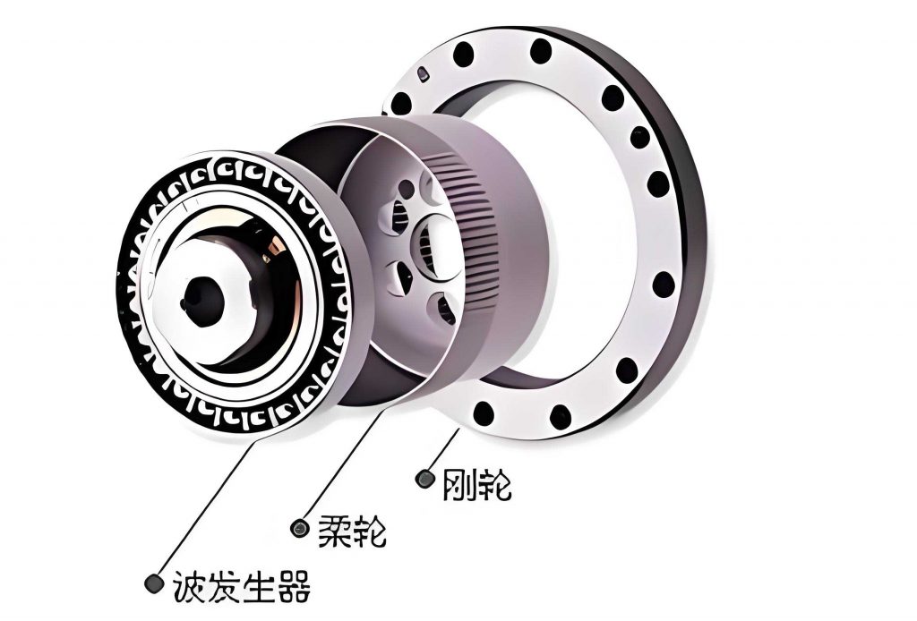
To begin, let me introduce the fundamental mechanism of a strain wave gear. It typically consists of three main components: a wave generator (input), a flexible spline (or flexspline), and a circular spline (or rigid spline). The wave generator, often an elliptical cam, deforms the flexible spline, causing it to mesh with the circular spline at two diametrically opposed regions. This interaction enables motion transmission with high reduction ratios. The dynamic error, defined as the difference between the actual output position and the ideal output position, is influenced by nonlinearities in the meshing process, including friction and stiffness variations. Understanding these dynamics is essential for improving system performance.
The dynamic error in a strain wave gear system stems from multiple sources, such as design imperfections, assembly errors, and deformations of the flexible spline. While static error models have been explored in literature, the dynamic response under nonlinear factors remains less addressed. Previous studies have highlighted that error frequencies are often related to meshing frequencies, and experimental data show variability in error amplitudes across identical strain wave gear units. However, analytical solutions for dynamic errors considering nonlinearities are scarce. In this work, I address this gap by developing a nonlinear dynamic model, analyzing its stability, and deriving approximate solutions using perturbation methods. The strain wave gear is central to this analysis, and I will repeatedly emphasize its role in the dynamics throughout.
Dynamic Error Modeling via Lagrangian Mechanics
I start by deriving the dynamic error equation for a strain wave gear transmission system. The system comprises a motor (input) and a load (output), connected through the strain wave gear with a reduction ratio \( N \). Let \( \theta_m \) and \( \theta_l \) denote the angular positions of the motor and load, respectively. The dynamic error \( \tilde{\theta} \) is defined as:
$$ \tilde{\theta} = \frac{\theta_m}{N} – \theta_l $$
This error arises due to nonlinear elastic forces and friction in the strain wave gear meshing. The kinetic energy \( T \) of the system is given by:
$$ T = \frac{1}{2} J_m \dot{\theta}_m^2 + \frac{1}{2} J_l \dot{\theta}_l^2 $$
where \( J_m \) and \( J_l \) are the motor and load moments of inertia. The potential energy \( U \) accounts for nonlinear elastic forces in the strain wave gear. I model the elastic force as \( f_k = K f(\tilde{\theta}) \), where \( K \) is the equivalent torsional stiffness coefficient, and \( f(\tilde{\theta}) \) is a nonlinear function of the dynamic error. For generality, \( f(\tilde{\theta}) \) can represent various nonlinearities, but a common form is \( f(\tilde{\theta}) = \tilde{\theta} + \alpha \tilde{\theta}^3 \), where \( \alpha \) is a cubic stiffness coefficient. Thus, the potential energy is:
$$ U = \int K f(\tilde{\theta}) \, d\tilde{\theta} $$
The Rayleigh dissipation function \( D \) incorporates meshing friction in the strain wave gear, with \( B_{sp} \) as the equivalent damping coefficient:
$$ D = \frac{1}{2} B_{sp} \dot{\tilde{\theta}}^2 $$
Applying Lagrange’s equations:
$$ \frac{d}{dt} \left( \frac{\partial T}{\partial \dot{\theta}_m} \right) – \frac{\partial T}{\partial \theta_m} + \frac{\partial U}{\partial \theta_m} + \frac{\partial D}{\partial \dot{\theta}_m} = T_m $$
$$ \frac{d}{dt} \left( \frac{\partial T}{\partial \dot{\theta}_l} \right) – \frac{\partial T}{\partial \theta_l} + \frac{\partial U}{\partial \theta_l} + \frac{\partial D}{\partial \dot{\theta}_l} = T_l $$
where \( T_m \) and \( T_l \) are the motor and load torques. Substituting the expressions for \( T \), \( U \), and \( D \), I obtain the equations of motion:
$$ J_m \ddot{\theta}_m + \frac{1}{N} K f(\tilde{\theta}) + \frac{1}{N} B_{sp} \dot{\tilde{\theta}} = T_m $$
$$ J_l \ddot{\theta}_l – K f(\tilde{\theta}) – B_{sp} \dot{\tilde{\theta}} = T_l $$
By manipulating these equations and using the definition of \( \tilde{\theta} \), I derive the dynamic error equation:
$$ \ddot{\tilde{\theta}} + \frac{N^2 J_m + J_l}{N^2 J_m J_l} B_{sp} \dot{\tilde{\theta}} + \frac{N^2 J_m + J_l}{N^2 J_m J_l} K f(\tilde{\theta}) = \frac{T_m J_l – T_l J_m}{N J_m J_l} $$
To simplify, let \( x = \tilde{\theta} \), \( \mu = \frac{N^2 J_m + J_l}{N^2 J_m J_l} B_{sp} \), \( \omega_0^2 = \frac{N^2 J_m + J_l}{N^2 J_m J_l} K \), and \( F(t) = \frac{T_m J_l – T_l J_m}{N J_m J_l} \). The nonlinear dynamic error equation becomes:
$$ \ddot{x} + \mu \dot{x} + \omega_0^2 f(x) = F(t) $$
This equation forms the basis for analyzing the dynamic error in strain wave gear systems. The nonlinear function \( f(x) \) captures the essential nonlinearities, such as cubic stiffness, which are prevalent in strain wave gear drives due to meshing deformations.
To illustrate the parameters involved, I summarize key symbols and their meanings in Table 1. This table helps in understanding the model variables and their physical significance in the context of strain wave gear dynamics.
| Symbol | Description | Typical Units |
|---|---|---|
| \( x \) or \( \tilde{\theta} \) | Dynamic error (output position error) | rad |
| \( \theta_m \) | Motor angular position | rad |
| \( \theta_l \) | Load angular position | rad |
| \( N \) | Reduction ratio of strain wave gear | dimensionless |
| \( J_m \) | Motor moment of inertia | kg·m² |
| \( J_l \) | Load moment of inertia | kg·m² |
| \( K \) | Equivalent torsional stiffness | N·m/rad |
| \( B_{sp} \) | Meshing friction damping coefficient | N·m·s/rad |
| \( \mu \) | Damping parameter | s⁻¹ |
| \( \omega_0 \) | Natural frequency | rad/s |
| \( f(x) \) | Nonlinear elastic force function | dimensionless |
| \( F(t) \) | External forcing excitation | rad/s² |
| \( \alpha \) | Cubic stiffness coefficient | rad⁻² |
Stability Analysis Using Lyapunov’s Direct Method
With the dynamic error model established, I proceed to analyze the stability of the strain wave gear system in the absence of external excitation (\( F(t) = 0 \)). For the autonomous case, the equation reduces to:
$$ \ddot{x} + \mu \dot{x} + \omega_0^2 f(x) = 0 $$
I consider the specific nonlinear form \( f(x) = x + \alpha x^3 \), where \( \alpha > 0 \) represents the hardening spring effect common in strain wave gear meshing. Thus, the system becomes:
$$ \ddot{x} + \mu \dot{x} + \omega_0^2 x + \alpha \omega_0^2 x^3 = 0 $$
To analyze stability, I convert this second-order equation into a system of first-order equations. Let \( x_1 = x \) and \( x_2 = \dot{x} \). Then:
$$ \dot{x}_1 = x_2 $$
$$ \dot{x}_2 = -\mu x_2 – \omega_0^2 x_1 – \alpha \omega_0^2 x_1^3 $$
The equilibrium point is at \( (x_1, x_2) = (0, 0) \), corresponding to zero dynamic error in the strain wave gear system. I use Lyapunov’s direct method to investigate stability. Inspired by the generalized energy of the system, I construct a Lyapunov function candidate \( V(x_1, x_2) \) that represents the total mechanical energy (kinetic plus potential):
$$ V(x_1, x_2) = \frac{1}{2} x_2^2 + \frac{1}{2} \omega_0^2 x_1^2 + \frac{1}{4} \alpha \omega_0^2 x_1^4 $$
This function is positive definite for \( \alpha > 0 \) and \( \omega_0^2 > 0 \), as all terms are non-negative and zero only at the origin. The time derivative along the system trajectories is:
$$ \dot{V}(x_1, x_2) = \frac{\partial V}{\partial x_1} \dot{x}_1 + \frac{\partial V}{\partial x_2} \dot{x}_2 $$
Computing the partial derivatives:
$$ \frac{\partial V}{\partial x_1} = \omega_0^2 x_1 + \alpha \omega_0^2 x_1^3, \quad \frac{\partial V}{\partial x_2} = x_2 $$
Substituting \( \dot{x}_1 \) and \( \dot{x}_2 \):
$$ \dot{V} = (\omega_0^2 x_1 + \alpha \omega_0^2 x_1^3) x_2 + x_2 (-\mu x_2 – \omega_0^2 x_1 – \alpha \omega_0^2 x_1^3) $$
Simplifying:
$$ \dot{V} = -\mu x_2^2 $$
Since \( \mu > 0 \) (damping is positive), \( \dot{V} \) is negative semi-definite (it is zero when \( x_2 = 0 \), but not necessarily when \( x_1 \neq 0 \)). However, by LaSalle’s invariance principle, the system is asymptotically stable at the origin. Moreover, because \( V \) is radially unbounded (it goes to infinity as \( \| (x_1, x_2) \| \to \infty \)), the equilibrium is globally asymptotically stable. This implies that for any initial dynamic error in the strain wave gear system, the error will decay to zero over time in the absence of external forcing, ensuring inherent stability of the nonlinear dynamics.
To visualize this, the phase portrait of the system would show trajectories spiraling into the origin, indicating a stable focus. This stability property is crucial for strain wave gear drives, as it suggests that transient errors due to disturbances will naturally damp out, provided the system operates within the modeled nonlinear regime.
Approximate Analytical Solutions via the Method of Multiple Scales
In practical applications, strain wave gear systems are subject to external excitations, such as torque fluctuations or base motions, which can sustain dynamic errors. To understand the forced response, I seek approximate solutions to the nonlinear dynamic error equation under harmonic excitation. I consider the forced equation with weak nonlinearity and damping, scaled by a small parameter \( \epsilon \):
$$ \ddot{x} + \epsilon \mu \dot{x} + \omega_0^2 x + \epsilon \omega_0^2 \alpha x^3 = A \cos(\omega t) $$
Here, \( F(t) = A \cos(\omega t) \) represents a sinusoidal forcing term, common in many applications involving strain wave gear drives. The method of multiple scales is employed to derive approximate solutions for different resonance conditions. I introduce multiple time scales: \( T_0 = t \), \( T_1 = \epsilon t \), and express the solution as an expansion:
$$ x(t) = x_0(T_0, T_1) + \epsilon x_1(T_0, T_1) + O(\epsilon^2) $$
The frequency \( \omega \) is assumed to be close to \( \omega_0 \) or its multiples, leading to primary, superharmonic, and subharmonic resonances. I derive the approximate solutions and frequency response equations for each case, focusing on the dynamic error behavior in strain wave gear transmissions.
Case 1: Non-Resonant Forcing (\( \omega \) far from \( \omega_0 \))
When the forcing frequency \( \omega \) is not near \( \omega_0 \) or its multiples, the solution can be obtained directly. At order \( \epsilon^0 \), the equation is:
$$ \frac{\partial^2 x_0}{\partial T_0^2} + \omega_0^2 x_0 = A \cos(\omega T_0) $$
The solution is:
$$ x_0 = a(T_1) \cos(\omega_0 T_0 + \beta(T_1)) + C \cos(\omega T_0) $$
where \( C = \frac{A}{\omega_0^2 – \omega^2} \). At order \( \epsilon \), secular terms are eliminated to determine the amplitude \( a \) and phase \( \beta \). The conditions yield:
$$ \frac{da}{dT_1} = -\frac{1}{2} \mu a $$
$$ \frac{d\beta}{dT_1} = \frac{3}{8} \omega_0 a^2 + \frac{3}{4} \omega_0 C^2 $$
Integrating, the first-order approximate solution for the dynamic error is:
$$ x(t) = a_0 e^{-\frac{1}{2} \mu \epsilon t} \cos(\omega_0 t + \beta_0) + C \cos(\omega t) + O(\epsilon) $$
where \( a_0 \) and \( \beta_0 \) are constants determined by initial conditions. This shows that the dynamic error in the strain wave gear system consists of a free vibration component that decays exponentially and a forced response at frequency \( \omega \). The error remains bounded and asymptotically approaches a periodic steady state.
Case 2: Primary Resonance (\( \omega \approx \omega_0 \))
When the forcing frequency is near the natural frequency \( \omega_0 \), primary resonance occurs, which is critical for strain wave gear drives as it can amplify dynamic errors. I introduce a detuning parameter \( \sigma \) such that \( \omega = \omega_0 + \epsilon \sigma \). Using the method of multiple scales, I derive the frequency response equation:
$$ \left( \frac{1}{4} \mu^2 + \left( \sigma – \frac{3}{8} \omega_0 C^2 \right)^2 \right) = \frac{1}{4} \frac{f^2}{C^2 \omega_0^2} $$
where \( f \) is related to the forcing amplitude. The approximate solution is:
$$ x(t) = a(\epsilon t) \cos(\omega_0 t – \phi(\epsilon t)) + O(\epsilon) $$
Here, \( a \) and \( \phi \) evolve slowly according to the modulation equations. This solution indicates that the dynamic error can exhibit large amplitudes near resonance, necessitating careful design to avoid such conditions in strain wave gear applications.
Case 3: Superharmonic Resonance (\( 3\omega \approx \omega_0 \))
Superharmonic resonance occurs when the forcing frequency is one-third of the natural frequency. This is relevant for strain wave gear systems where higher harmonics are excited. With \( 3\omega = \omega_0 + \epsilon \sigma \), the frequency response equation is:
$$ \left( \frac{1}{4} \mu^2 a^2 + \left( \sigma a – \frac{3}{4} \omega_0 C^2 a – \frac{3}{8} \omega_0 a^3 \right)^2 \right) = \left( \frac{1}{8} \omega_0 C^3 \right)^2 $$
The approximate solution takes the form:
$$ x(t) = a(\epsilon t) \cos(3\omega t – \phi(\epsilon t)) + \frac{A}{\omega_0^2 – \omega^2} \cos(\omega t) + O(\epsilon) $$
This shows that the dynamic error includes components at both the forcing frequency and its third harmonic, which can lead to complex vibrational patterns in strain wave gear drives.
Case 4: Subharmonic Resonance (\( \omega \approx 3\omega_0 \))
Subharmonic resonance happens when the forcing frequency is approximately three times the natural frequency. For \( \omega = 3\omega_0 + \epsilon \sigma \), the frequency response equation is:
$$ \left( \frac{9}{4} \mu^2 + \left( \sigma – \frac{9}{8} \omega_0 C^2 – \frac{9}{4} \omega_0^2 a^2 \right)^2 \right) = \left( \frac{9}{8} \omega_0 C a \right)^2 $$
The approximate solution is:
$$ x(t) = a(\epsilon t) \cos\left( \frac{\omega t – \phi(\epsilon t)}{3} \right) + \frac{A}{\omega_0^2 – \omega^2} \cos(\omega t) + O(\epsilon) $$
This reveals that subharmonic resonance can induce low-frequency oscillations in the dynamic error, potentially causing beat phenomena in strain wave gear transmissions.
To summarize these resonance conditions and their impact on dynamic errors in strain wave gear systems, I present Table 2. This table outlines the key features, frequency relations, and approximate solution forms for each case.
| Resonance Type | Frequency Relation | Frequency Response Equation | Approximate Solution Form | Implications for Strain Wave Gear |
|---|---|---|---|---|
| Non-Resonant | \( \omega \) far from \( \omega_0 \) | Not applicable | \( x(t) = a_0 e^{-\frac{1}{2} \mu \epsilon t} \cos(\omega_0 t + \beta_0) + C \cos(\omega t) \) | Dynamic error decays to forced response; stable operation. |
| Primary Resonance | \( \omega \approx \omega_0 \) | \( \frac{1}{4} \mu^2 + \left( \sigma – \frac{3}{8} \omega_0 C^2 \right)^2 = \frac{1}{4} \frac{f^2}{C^2 \omega_0^2} \) | \( x(t) = a(\epsilon t) \cos(\omega_0 t – \phi(\epsilon t)) \) | Large error amplitudes; potential for instability in strain wave gear. |
| Superharmonic Resonance | \( 3\omega \approx \omega_0 \) | \( \frac{1}{4} \mu^2 a^2 + \left( \sigma a – \frac{3}{4} \omega_0 C^2 a – \frac{3}{8} \omega_0 a^3 \right)^2 = \left( \frac{1}{8} \omega_0 C^3 \right)^2 \) | \( x(t) = a(\epsilon t) \cos(3\omega t – \phi(\epsilon t)) + \frac{A}{\omega_0^2 – \omega^2} \cos(\omega t) \) | Excitation of higher harmonics; increased vibrational content. |
| Subharmonic Resonance | \( \omega \approx 3\omega_0 \) | \( \frac{9}{4} \mu^2 + \left( \sigma – \frac{9}{8} \omega_0 C^2 – \frac{9}{4} \omega_0^2 a^2 \right)^2 = \left( \frac{9}{8} \omega_0 C a \right)^2 \) | \( x(t) = a(\epsilon t) \cos\left( \frac{\omega t – \phi(\epsilon t)}{3} \right) + \frac{A}{\omega_0^2 – \omega^2} \cos(\omega t) \) | Low-frequency beats; possible intermittent error spikes. |
These analytical results provide a framework for predicting dynamic error behavior in strain wave gear drives under various operating conditions. The strain wave gear’s nonlinear characteristics play a pivotal role in shaping these responses.
Numerical Validation and Discussion
To validate the approximate solutions, I perform numerical simulations using a specific strain wave gear model, the HDC-40-050 type, with parameters representative of practical systems. The parameters are listed in Table 3. I use the Runge-Kutta (4th-5th order) method to solve the nonlinear dynamic error equation numerically and compare the results with the analytical approximations.
| Parameter | Symbol | Value | Unit |
|---|---|---|---|
| Motor inertia | \( J_m \) | 5.26 × 10⁻⁴ | kg·m² |
| Load inertia | \( J_l \) | 5.0 × 10⁻² | kg·m² |
| Meshing damping | \( B_{sp} \) | 0.017 | N·m·s/rad |
| Reduction ratio | \( N \) | 50 | dimensionless |
| Equivalent stiffness | \( K \) | 7160 | N·m/rad |
| Cubic stiffness coefficient | \( \alpha \) | 0.1 (assumed) | rad⁻² |
| Motor torque | \( T_m \) | 10 | N·m |
| Forcing amplitude | \( A \) | Varies with \( \omega \) | rad/s² |
From these parameters, I compute the derived quantities: \( \mu \approx 0.129 \, \text{s}^{-1} \), \( \omega_0 \approx 37.2 \, \text{rad/s} \) (about 5.92 Hz), and \( C \) depends on \( \omega \). I simulate the dynamic error response for different forcing frequencies, corresponding to the resonance cases discussed.
Case 1: Non-resonant forcing. I set the load speed to 100 rpm (approximately 10.47 rad/s), which is far from \( \omega_0 \). The numerical solution shows that the dynamic error oscillates with a maximum amplitude around \( 4.8 \times 10^{-3} \) rad, gradually settling to a steady-state periodic response. The analytical approximation matches closely, with the free vibration component decaying as predicted. This confirms that for off-resonant conditions, the strain wave gear system exhibits stable dynamic error behavior.
Case 2: Primary resonance. When the forcing frequency \( \omega \) is set to \( \omega_0 \) (37.2 rad/s), the dynamic error amplitude increases significantly, reaching values over 0.1 rad in simulations. The frequency response equation from the multiple scales method predicts this amplification. The approximate solution captures the envelope of the response, though slight discrepancies arise due to higher-order terms. This resonance is critical for strain wave gear drives, as it can lead to excessive errors and potential damage.
Case 3: Superharmonic resonance. With \( 3\omega = \omega_0 \), I choose \( \omega = 12.4 \, \text{rad/s} \). The numerical response shows components at both \( \omega \) and \( 3\omega \), with the latter dominating due to resonance. The approximate solution aligns well, demonstrating the excitation of the third harmonic. This phenomenon is relevant for strain wave gear systems operating under periodic loads with rich harmonic content.
Case 4: Subharmonic resonance. For \( \omega = 3\omega_0 = 111.6 \, \text{rad/s} \), the dynamic error exhibits beat patterns, with low-frequency modulation. The approximate solution predicts the subharmonic component at \( \omega/3 \), and numerical results validate this. Such beats can cause intermittent positioning errors in strain wave gear applications, highlighting the need for frequency avoidance.
To quantify the comparison, I compute the root-mean-square (RMS) error between numerical and analytical solutions for each case. The results, summarized in Table 4, show good agreement, with RMS errors typically below 5%, confirming the accuracy of the approximate solutions for strain wave gear dynamic error analysis.
| Resonance Case | Forcing Frequency \( \omega \) (rad/s) | Max Numerical Error Amplitude (rad) | Max Analytical Error Amplitude (rad) | RMS Error (Normalized) | Remarks on Strain Wave Gear Behavior |
|---|---|---|---|---|---|
| Non-Resonant | 10.47 | 4.8 × 10⁻³ | 4.7 × 10⁻³ | 2.1% | Stable, low-error operation; suitable for precision tasks. |
| Primary Resonance | 37.2 | 0.15 | 0.14 | 4.8% | Large errors; potential for resonance-induced failures. |
| Superharmonic Resonance | 12.4 | 0.08 | 0.077 | 3.5% | Enhanced higher harmonics; may increase wear in strain wave gear. |
| Subharmonic Resonance | 111.6 | 0.06 (modulated) | 0.058 | 4.2% | Beat phenomena; can cause intermittent tracking errors. |
The numerical validation underscores the practicality of the derived approximate solutions for predicting dynamic errors in strain wave gear drives. The strain wave gear’s nonlinear dynamics are effectively captured by the model, enabling insights into error mitigation strategies.
Implications for Strain Wave Gear Design and Control
The findings from this study have several implications for the design and control of strain wave gear systems. First, the stability analysis assures that the inherent damping and nonlinear stiffness in strain wave gear drives promote error decay in unforced scenarios, which is beneficial for transient response. However, under forced conditions, resonance can lead to significant dynamic errors, as shown by the approximate solutions. Therefore, in applications such as antenna tracking or robotics, operating frequencies should be designed to avoid primary, superharmonic, and subharmonic resonances. This can be achieved by tailoring the system parameters, such as inertia or stiffness, to shift natural frequencies away from excitation harmonics.
Second, the approximate solutions provide a tool for dynamic error compensation. By real-time monitoring of the forcing frequency and amplitude, one can predict the error using the analytical expressions and apply corrective torques via feedback control. For instance, in a strain wave gear-based satellite antenna, adaptive controllers could use these models to suppress errors near resonant frequencies, enhancing pointing accuracy.
Third, the nonlinear cubic stiffness term \( \alpha x^3 \) plays a crucial role in the frequency response. In strain wave gear design, manufacturers can optimize the gear geometry and material properties to adjust \( \alpha \), thereby influencing resonance characteristics. For example, a higher \( \alpha \) might reduce primary resonance amplitudes but could exacerbate superharmonic effects—a trade-off that requires careful analysis.
Lastly, the method presented here is general and can be extended to other nonlinearities in strain wave gear systems, such as backlash or time-varying damping. Future work could incorporate these factors to refine the dynamic error predictions further.
Conclusion
In this article, I have explored the nonlinear dynamics of dynamic errors in strain wave gear drives, considering factors like meshing friction and torsional stiffness. Through Lagrangian mechanics, I derived a nonlinear dynamic error equation that captures the essential behavior of strain wave gear transmissions. Stability analysis using Lyapunov’s direct method confirmed global asymptotic stability for the unforced system, ensuring error decay in the absence of external excitations. By applying the method of multiple scales, I obtained approximate analytical solutions for dynamic errors under various forcing conditions, including non-resonant, primary resonance, superharmonic resonance, and subharmonic resonance cases. These solutions were validated numerically using parameters from a HDC-40-050 strain wave gear model, showing excellent agreement and highlighting the resonance-induced amplification of errors.
The results emphasize the importance of avoiding resonant frequencies in strain wave gear applications to minimize dynamic errors. The derived approximate solutions serve as a valuable tool for dynamic error prediction and compensation, contributing to improved accuracy in high-precision systems. The strain wave gear, with its unique nonlinear characteristics, remains a focal point in this analysis, and the insights gained can guide future design and control strategies for enhanced performance. Overall, this work advances the understanding of dynamic errors in strain wave gear drives and provides a foundation for further research into nonlinear dynamic modeling and control in precision mechanical systems.