
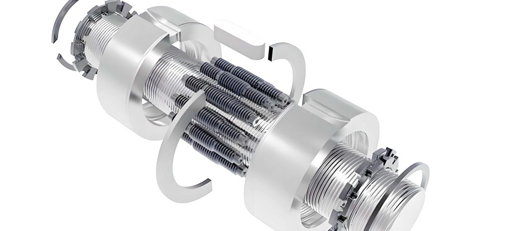
As an engineer deeply involved in the design and application of high-precision mechanical transmissions, I have consistently focused on the planetary roller screw. This remarkable mechanism is a transformative device that converts rotary motion into precise linear motion, comprising three core components: a central screw, multiple threaded rollers arranged around it, and an enclosing nut. Its brilliance lies in the harmonious integration of planetary motion with helical contact, offering superior load capacity, stiffness, efficiency, and longevity compared to more common alternatives like ball screws. Consequently, the planetary roller screw has become indispensable in demanding sectors such as aerospace, precision machine tools, robotics, and medical devices, where reliability and accuracy under heavy loads are non-negotiable.
The critical performance determinant for any planetary roller screw is the precise nature of its meshing contact—the way the threads of the screw, rollers, and nut engage. An excessive gap or backlash in this meshing leads to positional inaccuracy and challenges in servo-control. Conversely, excessive interference creates high preload, accelerating friction, wear, and ultimately reducing the system’s service life. Therefore, achieving and controlling the optimal meshing state is not merely a design goal but a fundamental requirement for high-performance planetary roller screw operation. My work centers on developing a robust, computationally efficient method to model this complex spatial contact and provide a clear path to eliminate the interference often encountered during assembly.
The three-dimensional, helical nature of the contact in a planetary roller screw defies simple two-dimensional analysis. To accurately describe it, one must begin by establishing a comprehensive spatial coordinate system. The primary fixed coordinate system is denoted as $$O(x, y, z)$$. From this, we derive the roller coordinate system $$O_R(x_R, y_R, z_R)$$, the screw coordinate system (aligned with the fixed system for the screw’s helical surface), and the nut coordinate system (also aligned with the fixed system for the nut’s helical surface). A key parameter is the center distance, $$a$$, which is the distance between the axes of the roller and the screw. For the initial theoretical design, this is often simply the sum of the nominal pitch radii: $$a = r_r + r_s$$, where $$r_r$$ and $$r_s$$ are the pitch radii of the roller and screw, respectively.
The foundation of meshing analysis lies in the mathematical definition of the helical surfaces. The thread profiles for the screw, nut, and roller are typically trapezoidal. For the roller, which often features a rounded crest, its left-side flank surface can be generated from a circular arc. Let us define the parameters: $$P_0$$ is the nominal pitch, $$R_r$$ is the radius of the roller thread profile arc, and $$\beta$$ is the thread half-angle. A point on the roller’s generating arc is parameterized by $$u_r$$. The coordinates of this point in the roller’s cross-sectional plane are:
$$
\begin{align*}
x_{rM}(u_r) &= R_r \sin u_r – R_r \sin \beta + r_r \\
y_{rM}(u_r) &= 0 \\
z_{rM}(u_r) &= -\frac{P_0}{4} + R_r \cos \beta – R_r \cos u_r
\end{align*}
$$
When this generating line undergoes a screw motion around the roller’s axis $$z_R$$, it sweeps out the complete helical surface. Introducing the rotation angle $$\theta_r$$ and the roller lead $$P_r = P_0$$, the parametric equations for the roller’s left flank surface in its own coordinate system become:
$$
\begin{align*}
x_r(u_r, \theta_r) &= (R_r \sin u_r – R_r \sin \beta + r_r) \cos \theta_r \\
y_r(u_r, \theta_r) &= (R_r \sin u_r – R_r \sin \beta + r_r) \sin \theta_r \\
z_r(u_r, \theta_r) &= -\frac{P_0}{4} + R_r \cos \beta – R_r \cos u_r + \frac{P_r \theta_r}{2\pi}
\end{align*}
$$
The surfaces for the screw and nut are simpler, generated from straight lines. For the screw’s right-side flank, using parameter $$u_s$$ and recognizing its multi-start nature (number of starts = $$n_s$$, lead $$P_s = n_s P_0$$), the equations in the fixed/screw coordinate system are:
$$
\begin{align*}
x_s(u_s, \theta_s) &= (u_s \cos \beta + r_s) \cos \theta_s \\
y_s(u_s, \theta_s) &= (u_s \cos \beta + r_s) \sin \theta_s \\
z_s(u_s, \theta_s) &= \frac{P_0}{4} + u_s \sin \beta + \frac{P_s \theta_s}{2\pi}
\end{align*}
$$
Similarly, for the nut’s right-side flank (number of starts = $$n_n$$, lead $$P_n = n_n P_0$$), the equations are:
$$
\begin{align*}
x_n(u_n, \theta_n) &= (u_n \cos \beta + r_n) \cos \theta_n \\
y_n(u_n, \theta_n) &= (u_n \cos \beta + r_n) \sin \theta_n \\
z_n(u_n, \theta_n) &= -\frac{P_0}{4} + u_n \sin \beta + \frac{P_n \theta_n}{2\pi}
\end{align*}
$$
The transformation between the roller coordinate system and the fixed system is a simple translation along the x-axis by the center distance $$a$$:
$$
\begin{bmatrix} x \\ y \\ z \\ 1 \end{bmatrix} =
\begin{bmatrix}
1 & 0 & 0 & a \\
0 & 1 & 0 & 0 \\
0 & 0 & 1 & 0 \\
0 & 0 & 0 & 1
\end{bmatrix}
\begin{bmatrix} x_R \\ y_R \\ z_R \\ 1 \end{bmatrix}
$$
Solving the continuous spatial meshing conditions for these helical surfaces analytically is exceptionally complex. To overcome this, I employ a discrete numerical approach that is both accurate and computationally efficient. The core idea is to sample the potential contact region on the transverse plane (the X-Y plane) and then calculate the axial separation of the two helical surfaces at each sample point. The point with the smallest axial separation defines the meshing point, and the value of this separation indicates the state of meshing: negative for interference, positive for clearance, and zero for ideal contact. The following table summarizes the step-by-step algorithm for the screw-roller pair analysis.
| Step | Action | Mathematical Description / Purpose |
|---|---|---|
| 1 | Discretize the Contact Zone | Define a grid of points $$P_{RSi}(x_{RSi}, y_{RSi})$$ in the X-Y plane within the shadowed potential contact region between the screw and roller pitch circles. |
| 2 | Calculate Axial Coordinates for Roller | For each point $$P_{RSi}$$, solve for parameters $$u_r$$ and $$\theta_r$$ that satisfy $$x_r(u_r, \theta_r)=x_{RSi}$$ and $$y_r(u_r, \theta_r)=y_{RSi}$$. Substitute back to get the axial coordinate $$z_{r,i}$$. |
| 3 | Calculate Axial Coordinates for Screw | For the same point $$P_{RSi}$$, solve for parameters $$u_s$$ and $$\theta_s$$ that satisfy $$x_s(u_s, \theta_s)=x_{RSi}$$ and $$y_s(u_s, \theta_s)=y_{RSi}$$. Substitute back to get the axial coordinate $$z_{s,i}$$. |
| 4 | Compute Axial Separation | Calculate the axial distance at point $$i$$: $$\Delta z_i = z_{r,i} – z_{s,i}$$. A negative $$\Delta z_{min}$$ indicates interference; a positive value indicates clearance. |
| 5 | Identify Meshing Point | The point corresponding to $$\Delta z_{min}$$ is the actual meshing point. Its transverse coordinates $$(x_m, y_m)$$ define the contact location. |
| 6 | Iterate for Design | Adjust geometric parameters (e.g., $$r_s$$, $$r_n$$) and repeat Steps 1-5 until the desired $$\Delta z_{min}$$ (e.g., ~0) is achieved. |
To validate the accuracy of this discrete method, I conducted a comparative study using a specific planetary roller screw design and a commercial CAD software’s interference detection tool. The nominal design parameters are listed below.
| Geometric Parameter | Screw | Roller | Nut |
|---|---|---|---|
| Pitch Diameter (mm) | 19.5 | 6.5 | 32.5 |
| Pitch, $$P_0$$ (mm) | 1 | 1 | 1 |
| Number of Starts / Lead (mm) | 5 / 5 | 1 / 1 | 5 / 5 |
| Thread Half-Angle, $$\beta$$ | 45° | 45° | 45° |
| Profile Radius (mm) | – | 3.0 | – |
Using the theoretical center distance $$a = r_r + r_s = 13.0 \text{ mm}$$, my algorithm predicted significant interference. To find the condition for zero clearance, I iteratively adjusted the screw’s pitch diameter. The virtual assembly in CAD reported interference volume, while my method computed the minimum axial gap. The results, perfectly correlated, are shown in the next table. This confirms that my discrete calculation method can achieve sub-micron precision (down to $$10^{-5}$$ mm) in determining the meshing state, fully meeting practical engineering requirements.
| Screw Pitch Diameter (mm) | CAD Interference Volume (mm³) | Proposed Method, $$\Delta z_{min}$$ (mm) | Meshing State |
|---|---|---|---|
| 19.50000 | 2.170 | -0.02070 | Strong Interference |
| 19.45860 | ~5.46e-9 | -3.13e-5 | Near-Zero Interference |
| 19.45854 | ~4e-11 | -1.25e-6 | Micro Interference |
| 19.45852 | 0.0 | +8.75e-6 | Micro Clearance |
The analysis conclusively demonstrates that assembling a planetary roller screw with theoretical pitch diameters and center distance leads to substantial interference. This is a fundamental characteristic of its spatial gearing geometry, not a manufacturing defect. The left plot below shows the calculated axial interference distribution for the nominal screw diameter (19.5 mm), revealing a broad area of deep interference. The meshing point for this nominal case was found at $$P_{xy} = (9.7648, 0.3191)$$ in the transverse plane.
The solution to this problem is elegant and practical: controlled adjustment of the pitch diameters. By reducing the screw’s pitch diameter to an optimized value (e.g., ~19.4585 mm in this case), the interference is completely eliminated, achieving near-ideal point contact. Crucially, this adjustment does not alter the transverse coordinates of the meshing point. As shown in the right plot and confirmed by calculations, the meshing point remains at $$P’_{xy} = (9.7648, 0.3191)$$. This is vitally important because it means the kinematic relationship—the fundamental motion transfer function of the planetary roller screw—remains unchanged. The adjustment only corrects the axial positioning of the helical surfaces relative to each other. The relationship can be summarized as:
$$
\text{Adjust } r_s \rightarrow \text{Eliminates Interference, } \Delta z_{min} \approx 0 \quad \text{while} \quad P_{xy} = \text{constant}
$$
In contrast, the meshing between the roller and the nut with theoretical parameters typically does not show inherent interference. This provides the designer with a separate control knob. The nut’s pitch diameter can be intentionally adjusted slightly to introduce a specific preload (negative clearance) or a controlled backlash (positive clearance) between the rollers and the nut, independently of the screw-roller interface. This enables the tuning of the overall system’s rigidity and preload without affecting its kinematics.
In practical manufacturing, this method translates directly into a precision machining guideline. Instead of targeting the theoretical pitch diameter for the screw, the drawing specifies the optimized, slightly smaller diameter calculated through this meshing analysis. For the nut, the target diameter is adjusted based on the desired system preload. This approach has been successfully implemented, transforming the assembly of planetary roller screw devices from a forced, interfering fit to a smooth, precise engagement, thereby ensuring optimal performance and longevity.
In conclusion, the discrete numerical method for analyzing the spatial meshing of a planetary roller screw provides a powerful and precise tool for designers. It accurately quantifies meshing interference or clearance, enabling the determination of critical manufacturing dimensions. The systematic adjustment of pitch diameters, particularly the screw’s, is the key to eliminating assembly interference while preserving the correct kinematics of the mechanism. This methodology bridges the gap between theoretical design and manufacturable, high-performance planetary roller screw systems, ensuring they deliver on their promise of high load capacity, precision, and durability in the most demanding applications.