
In modern industrial robotics, the rotary vector reducer plays a critical role in ensuring precise motion control and high torque transmission. The rotation error of a rotary vector reducer, defined as the deviation between the theoretical and actual output angles, directly impacts the performance and accuracy of robotic systems. This error arises from manufacturing tolerances and assembly inaccuracies in key components. In this study, we address the challenge of efficiently predicting the rotation error for rotary vector reducers, particularly the RV-40E type, to facilitate parts matching in production environments where manufacturing capabilities may be limited. Traditional methods rely on virtual prototyping, which is computationally expensive and time-consuming, making it unsuitable for real-time selection and assembly processes. Therefore, we propose a novel prediction method based on the Kriging model, a surrogate modeling technique that approximates the relationship between input parameters and output errors with high accuracy and efficiency.
The rotary vector reducer, often abbreviated as RV reducer, is a precision gear mechanism that combines planetary gear and cycloidal pin wheel transmissions. Its compact design, high reduction ratio, and low backlash make it ideal for applications in industrial robots, aerospace, and automation. However, the rotation error of a rotary vector reducer is sensitive to geometric deviations in components such as the pin gear radius, crankshaft eccentricity, pin gear center circle radius, and cycloidal wheel modifications. Accurately predicting this error is essential for quality control and assembly optimization. Our approach leverages the Kriging model to create a fast and reliable prediction tool, reducing the dependency on lengthy virtual prototype simulations. By integrating optimal Latin hypercube sampling, expectation improvement criteria, and particle swarm optimization, we develop a robust model that can be deployed in manufacturing settings for rapid parts matching.
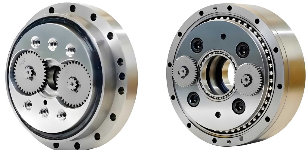
To understand the rotation error in a rotary vector reducer, we first analyze its structural principles. The RV-40E reducer consists of an input shaft, planetary gears, crankshafts, cycloidal wheels, pin gears, a pin gear housing, and an output planetary frame. The transmission process involves two stages: the primary planetary gear reduction and the secondary cycloidal pin wheel reduction. The rotation error, denoted as \(\phi_{er}\), is calculated using the formula:
$$ \phi_{er} = \frac{\phi_{in}}{i} – \phi_{out} $$
where \(\phi_{in}\) is the input angle, \(\phi_{out}\) is the actual output angle, and \(i\) is the transmission ratio, which for the RV-40E reducer is 121. The primary sources of error are geometric inaccuracies in the secondary cycloidal stage, as errors from the planetary stage are attenuated by the reduction ratio. We focus on five key influencing factors: pin gear radius error \(\delta_{rrp}\), pin gear center circle radius error \(\delta_{rp}\), crankshaft eccentricity error \(\delta_a\), cycloidal wheel equidistant modification amount \(\Delta_{rrp}\), and cycloidal wheel shift modification amount \(\Delta_{rp}\). These parameters are normalized to a range of [0,1] for modeling convenience, as shown in the following table summarizing their tolerance limits.
| Parameter | Symbol | Lower Limit (mm) | Upper Limit (mm) | Normalized Range |
|---|---|---|---|---|
| Pin Gear Radius | \(\delta_{rrp}\) | 4.01 | 4.03 | [0,1] |
| Pin Gear Center Circle Radius | \(\delta_{rp}\) | 82.005 | 82.015 | [0,1] |
| Crankshaft Eccentricity | \(\delta_a\) | 1.51 | 1.53 | [0,1] |
| Cycloidal Wheel Equidistant Modification | \(\Delta_{rrp}\) | 0.016 | 0.048 | [0,1] |
| Cycloidal Wheel Shift Modification | \(\Delta_{rp}\) | 0.026 | 0.078 | [0,1] |
The material properties of components also affect the rotation error due to elastic deformations under load. For instance, the cycloidal wheel and pin gears are made of alloy steels with specific elastic moduli and densities. However, for simplicity in initial modeling, we treat these as constants and later incorporate flexibility in virtual prototypes. The relationship between these factors and the rotation error is nonlinear and coupled, necessitating a sophisticated modeling approach. In this context, the rotary vector reducer serves as a complex system where traditional analytical methods fall short, prompting the use of surrogate models like Kriging.
To generate data for building the Kriging model, we develop a virtual prototype of the RV-40E rotary vector reducer using multi-body dynamics software. The process involves creating 3D models in CREO, importing them into ADAMS, and replacing rigid components with flexible bodies modeled in ANSYS for critical parts like the crankshaft, cycloidal wheel, and pin gears. This hybrid approach captures both geometric errors and elastic deformations, providing realistic simulation results. The virtual prototype is validated through experimental tests on physical reducers, where rotation errors measured on a test bench are compared with simulation outputs. The results show a relative error of less than 5%, confirming the reliability of the virtual prototype for generating training data. The table below presents a comparison of simulation and experimental results for three sample reducers, highlighting the accuracy of the virtual prototype.
| Sample | Pin Gear Radius (mm) | Crankshaft Eccentricity (mm) | Simulated Error (arc-min) | Experimental Error (arc-min) | Relative Error (%) |
|---|---|---|---|---|---|
| 1 | 4.018 | 1.519 | 1.137 | 1.098 | 3.43 |
| 2 | 4.027 | 1.515 | 2.267 | 2.182 | 3.75 |
| 3 | 4.012 | 1.525 | 1.090 | 1.041 | 4.50 |
With the virtual prototype established, we proceed to construct the Kriging model for predicting the rotation error of the rotary vector reducer. The Kriging model is a spatial interpolation technique that combines a global regression model with a localized stochastic process. For a set of input variables \(\mathbf{x} = [a, b, c, d, e]\), where \(a = \delta_{rrp}\), \(b = \delta_{rp}\), \(c = \delta_a\), \(d = \Delta_{rrp}\), and \(e = \Delta_{rp}\), the predicted response \(y(\mathbf{x})\) is given by:
$$ y(\mathbf{x}) = \mathbf{f}^T(\mathbf{x}) \boldsymbol{\beta} + \mathbf{r}^T(\mathbf{x}) \boldsymbol{\gamma} $$
Here, \(\mathbf{f}(\mathbf{x})\) is a vector of basis functions representing the global trend, \(\boldsymbol{\beta}\) are regression coefficients, \(\mathbf{r}(\mathbf{x})\) is a correlation vector between the prediction point and sample points, and \(\boldsymbol{\gamma}\) are weights for the stochastic part. The basis functions include constant, linear, and quadratic terms, such as \(f_1(\mathbf{x}) = 1\), \(f_2(\mathbf{x}) = a\), \(f_3(\mathbf{x}) = b\), up to \(f_{21}(\mathbf{x}) = e^2\), ensuring flexibility in capturing nonlinearities. The correlation function is Gaussian, defined as:
$$ r(\mathbf{x}_i, \mathbf{x}_j) = \exp\left[ -\sum_{l=1}^{5} \theta_l (x_i^{(l)} – x_j^{(l)})^2 \right] $$
where \(\theta_l\) are hyperparameters that control the influence of each dimension. To estimate these parameters, we use maximum likelihood estimation, optimizing the log-likelihood function:
$$ \ln L \approx -\frac{1}{2} \ln(\sigma^2) – \frac{1}{2} \ln(|\mathbf{R}|) $$
with \(\sigma^2\) being the process variance and \(\mathbf{R}\) the correlation matrix of sample points.
We begin by generating an initial sample set using optimal Latin hypercube sampling (OLHS), which ensures uniform coverage of the five-dimensional parameter space. OLHS minimizes the sum of squared distances between points, as per the criterion:
$$ \sum_{i=1}^{n} \sum_{j=1}^{n} d_{ij}^2 = \min \sum_{i=1}^{n} \sum_{j=1}^{n} \sum_{l=1}^{5} (x_i^{(l)} – x_j^{(l)})^2 $$
where \(n = 50\) is the number of initial samples. For each sample point, we run the virtual prototype simulation to obtain the rotation error value, resulting in a dataset of 50 input-output pairs. This dataset is used to fit the initial Kriging model, yielding parameters \(\boldsymbol{\theta}\), \(\boldsymbol{\beta}\), and \(\boldsymbol{\gamma}\). The accuracy of the initial model is assessed using root mean square error (RMSE) and normalized maximum absolute error (NMAE):
$$ \text{RMSE} = \sqrt{\frac{\sum_{i=1}^{n} (y_i – \hat{y}_i)^2}{n}} $$
$$ \text{NMAE} = \max \left( \frac{|y_i – \hat{y}_i|}{n} \right) $$
where \(y_i\) are simulated errors and \(\hat{y}_i\) are predicted errors. The initial model shows RMSE = 3.7288 and NMAE = 0.1500, indicating room for improvement. Therefore, we implement an iterative refinement process using a double-point addition strategy.
To enhance the Kriging model for the rotary vector reducer, we employ two addition criteria: expected improvement (EI) and minimizing prediction (MP). The EI criterion targets global exploration by adding points where the potential for error reduction is highest, based on the expected improvement function:
$$ E[I(\mathbf{x})] = (y_{\text{min}} – \hat{y}(\mathbf{x})) \Phi\left( \frac{y_{\text{min}} – \hat{y}(\mathbf{x})}{s(\mathbf{x})} \right) + s(\mathbf{x}) \phi\left( \frac{y_{\text{min}} – \hat{y}(\mathbf{x})}{s(\mathbf{x})} \right) $$
Here, \(y_{\text{min}}\) is the minimum observed error, \(\hat{y}(\mathbf{x})\) is the predicted error, \(s(\mathbf{x})\) is the prediction standard deviation, and \(\Phi\) and \(\phi\) are the standard normal cumulative distribution and density functions, respectively. The MP criterion focuses on local exploitation by adding points where the prediction variance is minimized:
$$ \mathbf{x}^* = \arg \min s^2(\mathbf{x}) $$
with \(s^2(\mathbf{x})\) computed as:
$$ s^2(\mathbf{x}) = \sigma^2 \left(1 – \mathbf{u}^T (\mathbf{F}^T \mathbf{R}^{-1} \mathbf{F})^{-1} \mathbf{u} – \mathbf{r}^T(\mathbf{x}) \mathbf{R}^{-1} \mathbf{r}(\mathbf{x}) \right) $$
where \(\mathbf{u} = \mathbf{F}^T \mathbf{R}^{-1} \mathbf{r}(\mathbf{x}) – \mathbf{f}(\mathbf{x})\). We use particle swarm optimization (PSO) to accelerate the search for optimal addition points. PSO updates particle positions and velocities iteratively:
$$ \mathbf{v}_i^{(l)}(t+1) = \omega \mathbf{v}_i^{(l)}(t) + c_1 r_1 (p_i^{(l)}(t) – x_i^{(l)}(t)) + c_2 r_2 (g^{(l)}(t) – x_i^{(l)}(t)) $$
$$ x_i^{(l)}(t+1) = x_i^{(l)}(t) + v_i^{(l)}(t+1) $$
with inertia weight \(\omega = 1\), learning factors \(c_1 = c_2 = 2\), and random numbers \(r_1, r_2 \in [0,1]\). After each addition, we run the virtual prototype to obtain the new error value, update the sample set, and rebuild the Kriging model. This process continues for 54 iterations, resulting in a total of 104 sample points and a refined model with significantly improved accuracy.
The final Kriging model for the rotary vector reducer demonstrates high precision in predicting rotation errors. Below, we present the optimized parameters and accuracy metrics, showing a substantial reduction in error compared to the initial model.
| Parameter Type | Symbol | Values |
|---|---|---|
| Correlation Parameters | \(\boldsymbol{\theta}\) | \(\theta_1 = 39.036, \theta_2 = 50.000, \theta_3 = 28.558, \theta_4 = 25.786, \theta_5 = 50.000\) |
| Regression Coefficients | \(\boldsymbol{\beta}\) | \(\beta_1 = 0.668, \beta_2 = 0.371, \beta_3 = -0.429, \beta_4 = 0.829, \beta_5 = 0.414, \dots, \beta_{21} = -0.022\) |
| Stochastic Weights | \(\boldsymbol{\gamma}\) | \(\gamma_1 = -0.070, \gamma_2 = 0.123, \gamma_3 = 0.117, \dots, \gamma_{104} = 1.144\) |
| Model Stage | RMSE (arc-min) | NMAE (arc-min) |
|---|---|---|
| Initial Model (50 samples) | 3.7288 | 0.1500 |
| Final Model (104 samples) | 0.6350 | 0.0298 |
To validate the practical utility of our Kriging model for the rotary vector reducer, we compare its predictions with both virtual prototype simulations and experimental measurements. We select three additional sets of component parameters from a parts library, assemble them into RV-40E reducers, and measure the rotation errors using a test bench. The Kriging model predictions are generated in seconds, whereas virtual prototype simulations take hours. The results, summarized in the table below, confirm that the Kriging model achieves high accuracy with minimal computational time, making it suitable for real-time parts matching in production lines.
| Method | Time Required | Rotation Error Sample 1 (arc-min) | Rotation Error Sample 2 (arc-min) | Rotation Error Sample 3 (arc-min) |
|---|---|---|---|---|
| Experimental Test | 12.5 hours | 1.455 | 1.657 | 1.290 |
| Virtual Prototype Simulation | 1.5 hours | 1.427 | 1.641 | 1.279 |
| Kriging Model Prediction | 10 seconds | 1.422 | 1.648 | 1.270 |
The effectiveness of the Kriging model is further illustrated through a 3D surface plot showing the relationship between pin gear radius error, pin gear center circle radius error, and predicted rotation error, with other parameters fixed at mid-range values. This visualization highlights the nonlinear interactions and sensitivities, underscoring the complexity of the rotary vector reducer system. For instance, the rotation error tends to increase as both radius errors decrease, but the pattern is influenced by coupling effects. Such insights are valuable for designers and manufacturers in setting tolerance limits and prioritizing quality control measures.
In conclusion, our study presents a robust and efficient method for predicting the rotation error of rotary vector reducers using a Kriging model. By integrating virtual prototyping, optimal sampling, and iterative refinement with PSO acceleration, we develop a surrogate model that reduces prediction time from hours to seconds while maintaining high accuracy. This approach addresses the practical needs of manufacturers with limited production capabilities, enabling effective parts matching to achieve desired quality levels. The rotary vector reducer, as a key component in precision machinery, benefits from this predictive tool, which can be extended to other reducer types or mechanical systems with similar error sensitivities. Future work could incorporate additional factors such as thermal deformations, lubrication effects, or dynamic loads to further enhance model fidelity. Ultimately, the Kriging-based prediction method offers a scalable solution for improving the performance and reliability of rotary vector reducers in industrial applications.
The success of this method hinges on the careful selection of influencing factors and the iterative improvement of the surrogate model. We emphasize that the rotary vector reducer’s rotation error is a multifaceted problem requiring advanced modeling techniques. Our contributions include the development of a virtual prototype for data generation, the application of Kriging with double-point addition, and the validation through comparative analysis. As robotics and automation continue to advance, tools like this Kriging model will play a crucial role in optimizing the manufacturing and assembly of critical components like the rotary vector reducer.