
In recent years, quadruped robots have gained significant attention due to their exceptional adaptability to unstructured terrains, such as slopes, rough surfaces, and obstacles. However, navigating non-uniform slopes remains a challenge, as it requires balancing stability and foot-end mobility to prevent tipping or leg joint overextension. Traditional methods often focus on either maintaining a horizontal body posture or aligning with the slope surface, but these approaches can limit the robot dog’s ability to handle obstacles or irregular inclines. In this work, we propose a comprehensive pose optimization framework for quadruped robots operating on unstructured slopes. By estimating slope parameters from foot-end positions and analyzing key performance metrics like stability margin and foot-end workspace, we formulate a weighted objective function. This function is optimized using the Marine Predators Algorithm (MPA) to determine the optimal body displacement and pitch angle, enhancing both stability and obstacle-crossing capabilities. Through simulations in Webots and MATLAB, we validate that our method improves the quadruped robot’s performance across diverse slope scenarios, ensuring robust navigation in complex environments.
The core of our approach lies in addressing the limitations of existing strategies, which often prioritize stability at the expense of foot-end mobility. For instance, keeping the body horizontal on a slope can compress the front legs, reducing their effective workspace, while aligning the body with the slope may increase the risk of tipping. Our method dynamically adjusts the pose based on real-time terrain estimation, leveraging the robot dog’s kinematic model and environmental constraints. This not only maximizes stability but also ensures that the quadruped robot can traverse obstacles such as rocks or steps on inclines. By integrating these elements into a unified optimization process, we enable the quadruped robot to adapt seamlessly to varying slope conditions, making it more versatile for applications in search and rescue, exploration, and industrial inspections.
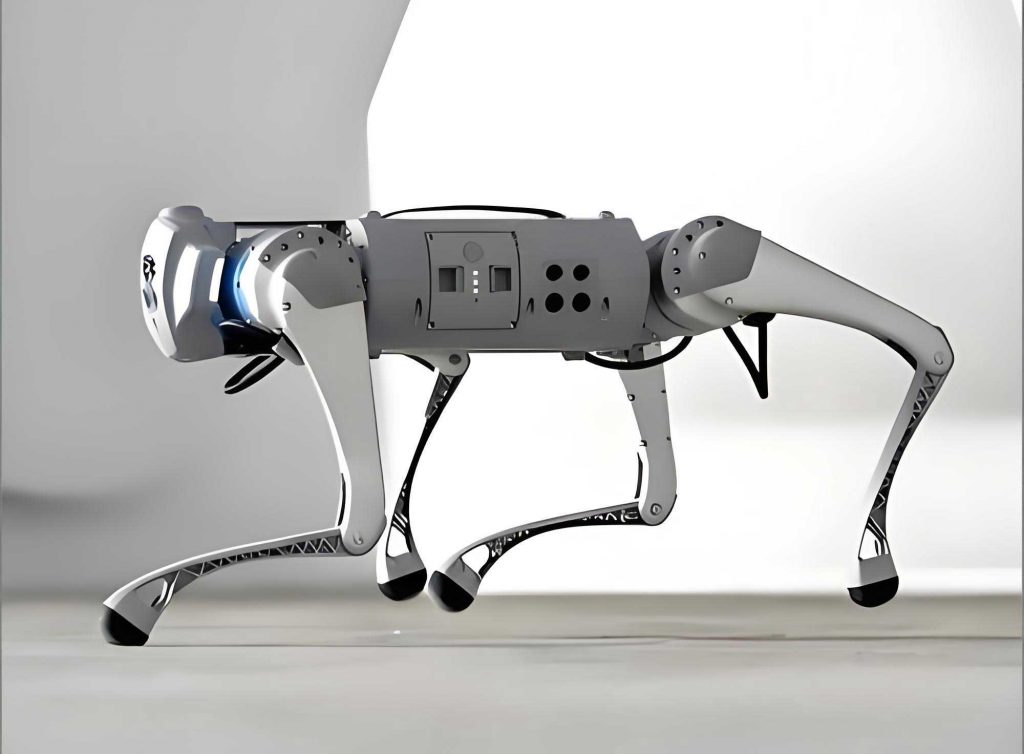
To begin, we model the quadruped robot with 12 degrees of freedom, distributed as three per leg: a side-swing joint, hip joint, and knee joint. The kinematic parameters, including link lengths and joint limits, are summarized in Table 1. The forward kinematics equation for the foot-end position in the body coordinate system is derived as follows: $$ \begin{bmatrix} p_x \\ p_y \\ p_z \end{bmatrix} = \begin{bmatrix} -l_3 \sin(\theta_2 + \theta_3) – l_2 \sin\theta_2 \\ l_3 \sin\theta_1 \cos(\theta_2 + \theta_3) + l_1 \cos\theta_1 + l_2 \cos\theta_2 \sin\theta_1 \\ l_1 \sin\theta_1 – l_3 \cos\theta_1 \cos(\theta_2 + \theta_3) – l_2 \cos\theta_1 \cos\theta_2 \end{bmatrix} $$ where $l_1$, $l_2$, and $l_3$ represent the lengths of the side-swing, thigh, and shank links, respectively, and $\theta_1$, $\theta_2$, $\theta_3$ are the joint angles. This model forms the basis for estimating slope parameters and analyzing the workspace of the robot dog.
| Parameter | Value |
|---|---|
| Body Length (L) | 0.361 m |
| Body Width (W) | 0.261 m |
| Side-Swing Link Length (l₁) | 0.0838 m |
| Thigh Link Length (l₂) | 0.2 m |
| Shank Link Length (l₃) | 0.2 m |
| Side-Swing Joint Angle Range (θ₁) | -0.802 to 0.802 rad |
| Hip Joint Angle Range (θ₂) | -1.05 to 4.19 rad |
| Knee Joint Angle Range (θ₃) | -2.70 to -0.92 rad |
For gait selection, we employ a static walk gait with a sequence of left hind leg → left front leg → right hind leg → right front leg, incorporating a quadruple support phase during transitions to enhance stability. This gait minimizes disturbances on unknown terrains, making it suitable for slope navigation. The robot dog’s coordinate systems, including the body frame {O_b}, hip joint frame {O_2}, and world frame {O_w}, are defined to facilitate transformations and pose adjustments. The homogeneous transformation matrix between these frames allows us to compute foot-end positions relative to the slope, which is crucial for parameter estimation.
Estimating the parameters of an unstructured slope is the first step in our pose optimization method. Since natural slopes are often irregular, we use the positions of three foot-ends in the world coordinate system to define a virtual slope plane. For example, if the next swing leg is leg 4, we use the foot-end positions of legs 1, 2, and 4 to form this plane. The normal vector $\zeta = (x_{cv}, y_{cv}, z_{cv})$ of the virtual slope is calculated using the cross product: $$ \zeta = \overrightarrow{p_{f1}p_{f2}} \times \overrightarrow{p_{f1}p_{f4}} $$ where the components are derived as: $$ x_{cv} = (y_{f2} – y_{f1}) \cdot (z_{f4} – z_{f1}) – (y_{f4} – y_{f1}) \cdot (z_{f2} – z_{f1}) $$ $$ y_{cv} = (z_{f2} – z_{f1}) \cdot (x_{f4} – x_{f1}) – (z_{f4} – z_{f1}) \cdot (x_{f2} – x_{f1}) $$ $$ z_{cv} = (x_{f2} – x_{1}) \cdot (y_{f4} – y_{f1}) – (x_{f4} – x_{f1}) \cdot (y_{f2} – y_{f1}) $$ The slope angle $\alpha$ is then found by computing the angle between the normal vector and the unit vector in the opposite direction of gravity $\nu = (0, 0, 1)$: $$ \alpha = \arccos\left( \frac{\zeta \cdot \nu}{|\zeta| \cdot |\nu|} \right) = \arccos\left( \frac{z_{cv}}{\sqrt{x_{cv}^2 + y_{cv}^2 + z_{cv}^2}} \right) $$ This angle $\alpha$ represents the inclination of the virtual slope, which the quadruped robot must adapt to.
Additionally, the forward direction angle $\gamma$, which is the projection of the robot’s heading onto the horizontal plane relative to the world x-axis, is determined using the midpoints of the foot-end projections. For instance, the midpoint between legs 1 and 2 is $p_{fm1} = \left( \frac{x_{f1} + x_{f2}}{2}, \frac{y_{f1} + y_{f2}}{2}, 0 \right)$, and similarly for legs 3 and 4. The angle $\gamma$ is computed as: $$ \gamma = \arccos\left( \frac{\overrightarrow{p_{fm2}p_{fm1}} \cdot \eta}{|\overrightarrow{p_{fm2}p_{fm1}}| \cdot |\eta|} \right) $$ where $\eta = (1, 0, 0)$ is the unit vector along the world x-axis. These estimated parameters, $\alpha$ and $\gamma, enable the quadruped robot to adjust its pose dynamically for improved performance on slopes.
Next, we analyze the slope motion performance of the robot dog, focusing on stability and foot-end mobility. Stability is quantified using the stability margin (SM), defined as the shortest distance from the projection of the center of gravity (CoG) to the edges of the support polygon formed by the supporting feet. For a quadruped robot in a static gait, the support polygon is a triangle during triple support phases. The distance $d_n$ from the CoG projection $P’_{cog}$ to each edge of the triangle is calculated using Heron’s formula: $$ d_n = \frac{2 \sqrt{p(p – a)(p – b)(p – c)}}{c} $$ where $a$, $b$, and $c$ are the distances from $P’_{cog}$ to the vertices of the triangle, and $p$ is the semi-perimeter. The stability margin is then: $$ SM = \min\{d_1, d_2, d_3\} $$ To maximize SM, we plan the CoG to lie within the double support triangle (DST) region, where support triangles overlap during leg swings, reducing the need for frequent CoG adjustments and enhancing overall stability.
Foot-end mobility is evaluated based on the feasible workspace, which represents the reachable area of the foot-end in the pitch plane (x-z plane) under environmental constraints. We use the Monte Carlo method to generate random joint angles within their limits and compute the corresponding foot-end positions via forward kinematics. The feasible workspace is constrained to exclude areas above the hip joint and adapt to slope conditions. It is divided into five boundary curves: negative boundary $\overset{\frown}{AB}$, positive boundary $\overset{\frown}{BC}$, concave boundary $\overset{\frown}{ED}$, lateral boundaries AE and CD, and environmental constraint boundary $\overset{\frown}{FG}$. These boundaries are fitted with fifth-degree polynomial functions: $$ f_i(x) = a_i x^5 + b_i x^4 + c_i x^3 + d_i x^2 + e_i x + g_i \quad \text{for } i = 1, 2, 3, 4 $$ where $f_1(x)$, $f_2(x)$, $f_3(x)$, and $f_4(x)$ correspond to the negative, positive, concave, and lateral boundaries, respectively. The coefficients are determined through curve fitting to model the workspace accurately.
The foot-end’s motion capability is characterized by the maximum reachable distance $\Delta l$ and maximum crossing height $\Delta h$ on the slope. When the robot adjusts its pose by a pitch angle $\phi$ and a CoG displacement $\Delta x_l$ along the forward direction, the homogeneous transformation matrix from the initial hip frame to the adjusted frame is: $$ T_{b}^{b’} = \begin{bmatrix} \cos\phi & \sin\phi & \Delta x \\ -\sin\phi & \cos\phi & -\Delta y \\ 0 & 0 & 1 \end{bmatrix} $$ where $\Delta x = \Delta x_l + \frac{L}{2} [\cos(\alpha – \phi) – \cos\alpha]$ and $\Delta y = \frac{L}{2} [\sin\alpha – \sin(\alpha – \phi)]$. The foot-end position in the adjusted frame is obtained as $p_b = (T_{b}^{b’})^{-1} p’_b$. The environmental constraint boundary in the hip frame is given by: $$ f_5(x) = \tan\phi \cdot (x – x_b) + z_b $$ The maximum reachable distance $\Delta l$ is the distance from the foot-end $p_b$ to the intersection point $p_{if}$ of $f_5(x)$ with the positive boundary $f_2(x)$: $$ \Delta l = \sqrt{(x_{if} – x_b)^2 + (z_{if} – z_b)^2} $$ The maximum crossing height $\Delta h$ is the minimum distance between the concave boundary $f_4(x)$ and the environmental constraint $f_5(x)$, found by solving for the zero derivative of the distance function $d(x) = f_4(x) – f_5(x)$: $$ \Delta h = \frac{ | \tan\phi \cdot (x_0 – x_b) – f_4(x_0) + z_b | }{ \sqrt{\tan^2\phi + 1} } $$ where $x_0$ is the x-coordinate where $d'(x) = 0$. These metrics are crucial for assessing the quadruped robot’s ability to overcome obstacles on slopes.
With the slope parameters and performance metrics defined, we formulate a pose optimization problem to determine the optimal CoG displacement $d_c$ and pitch angle $\phi$. The objective function combines three goals: maximizing foot-end mobility, stability margin, and minimizing the overturning risk. Foot-end mobility is expressed as a weighted sum: $$ O_1 = a \Delta l + b \Delta h $$ where $a$ and $b$ are weighting coefficients that vary based on the scenario—e.g., higher $a$ for obstacle-rich environments and higher $b$ for stability-focused cases. The stability margin $O_2$ is directly used as $SM$, and the overturning risk $O_3$ is approximated as $\phi^3 / 2$, reflecting the increased tipping tendency with larger pitch angles. The overall objective function is a weighted sum of these components: $$ J = \frac{1}{w_1 O_1 + w_2 O_2 + w_3 / O_3} $$ where $w_1$, $w_2$, and $w_3$ are weighting coefficients. Minimizing $J$ corresponds to maximizing performance, as $O_3$ is inversely related to stability.
| Parameter | Scenario 1 (Stability-Focused) | Scenario 2 (Mobility-Focused) |
|---|---|---|
| a | 0.5 | 0.4 |
| b | 0.5 | 0.6 |
| w₁ | 0.4 | 0.6 |
| w₂ | 0.5 | 0.3 |
| w₃ | 0.1 | 0.1 |
Constraints are applied to ensure feasible poses: the CoG displacement $d_c$ must be between 0 and the maximum allowed distance to the DST region, and the pitch angle $\phi$ must not exceed the slope angle $\alpha$ to prevent over-extension. Specifically: $$ C_1: 0 \leq d_c \leq x’_{com} – x^d_{com} $$ $$ C_2: 0 \leq \phi \leq \alpha $$ where $x’_{com}$ is the current CoG projection, and $x^d_{com}$ is the desired position in the DST region.
To solve this optimization problem, we employ the Marine Predators Algorithm (MPA), a metaheuristic inspired by predator-prey interactions in oceans. MPA uses Lévy and Brownian motions to explore the solution space efficiently. The algorithm initializes a population of prey individuals representing candidate solutions $(d_c, \phi)$, with positions bounded by the constraints. The fitness of each individual is evaluated using $J$. The optimization process is divided into three phases based on the iteration count $t_{iter}$ relative to the maximum iterations $t_{max}$. In the first phase (high velocity ratio, $t_{iter} < t_{max}/3$), prey movement is modeled as: $$ s_i = R_B \otimes (E_i – R_B \otimes P_i) $$ $$ P_i = P_i + l \cdot r(0,1) \otimes s_i $$ where $R_B$ is a Brownian motion vector, $E_i$ is the elite matrix (best solutions), $l=0.5$, and $\otimes$ denotes element-wise multiplication. In the second phase (equal velocity ratio, $t_{max}/3 < t_{iter} < 2t_{max}/3$), the update incorporates both Lévy ($R_L$) and Brownian motions: $$ s_i = (a \cdot R_L + b \cdot R_B) \otimes \left( a(E_i – R_L \otimes P_i) + b(R_B \otimes E_i – P_i) \right) $$ $$ P_i = (a \cdot P_i + b \cdot E_i) + l \cdot (a \cdot r(0,1) + b \cdot F_C) \otimes s_i $$ where $a$ and $b$ are exploration-exploitation coefficients, and $F_C = 1 – (t_{iter} / t_{max})^{2t_{iter} / t_{max}}$ is an adaptive factor. In the third phase (low velocity ratio, $2t_{max}/3 < t_{iter} < t_{max}$), the update relies on Lévy motion: $$ s_i = R_L \otimes (R_L \otimes E_i – P_i) $$ $$ P_i = E_i + l \cdot F_C \otimes s_i $$ After iterations, MPA outputs the optimal $d_{c,opt}$ and $\phi_{opt}$, which are used to adjust the robot’s pose via homogeneous transformations.
We validate our method through co-simulation in Webots and MATLAB, testing two scenarios: Scenario 1 emphasizes stability on irregular slopes with few obstacles, and Scenario 2 focuses on mobility with high obstacles. For Scenario 1, the weighting coefficients are set as in Table 2, and MPA converges within about 9 iterations, yielding $\phi_{opt}$ and $d_{c,opt}$ that enhance stability. The foot-end trajectory follows a smooth cycloidal path to minimize acceleration changes. Simulations show the quadruped robot traversing the slope steadily without tipping. In Scenario 2, the weights are adjusted to prioritize $\Delta h$ and $\Delta l$, and MPA converges similarly. The foot-end uses a rectangular trajectory scaled by $e = 0.85$ of the maximum values to avoid kinematic limits. The robot successfully climbs a 0.17 m obstacle on the slope, demonstrating improved obstacle-crossing capability.
In conclusion, our pose optimization method for quadruped robots on unstructured slopes effectively balances stability and foot-end mobility by leveraging real-time slope estimation and performance metrics. The use of MPA ensures efficient convergence to optimal poses, adapting to various terrain challenges. This approach enhances the robot dog’s versatility in non-uniform environments, paving the way for advanced applications in autonomous navigation. Future work could integrate dynamic gait adjustments and machine learning for faster adaptation.