
Quadruped robots, often referred to as robot dogs, have garnered significant attention due to their ability to traverse complex terrains inspired by biological counterparts. The unique leg structure of quadruped robots enables adaptation to various unstructured environments, but existing control algorithms, particularly those based on virtual model quadratic programming (QP), often overlook comprehensive terrain information, limiting stability and precision. This paper addresses these limitations by proposing an online terrain complexity estimation method using the robot’s proprioceptive system and enhancing the controller for improved stability. We integrate foot kinematics and centroid momentum feedback to design a terrain complexity estimation function, which combines terrain evaluation with dynamic performance assessment. The control algorithm incorporates this estimation to optimize both stance and swing phases: in the stance phase, external disturbance compensation and support force constraints are added, while in the swing phase, footstep planning and gait cycle adjustments are implemented. Validation through simulations with the Unitree A1 quadruped robot in Webots demonstrates enhanced stability on unstructured terrains.
The development of quadruped robots has advanced remarkably, with applications in industrial inspection, search and rescue, and exploration. However, maintaining stability on uneven terrain remains a challenge. Traditional control methods, such as virtual model control (VMC), often assume flat ground or simplified terrain models, leading to performance degradation in real-world scenarios. Our approach leverages the robot dog’s onboard sensors, including inertial measurement units (IMUs) and foot contact sensors, to continuously estimate terrain complexity and adapt control parameters accordingly. This enables the quadruped robot to dynamically adjust to obstacles, slopes, and other irregularities, ensuring robust locomotion.
Modeling of the Quadruped Robot
The quadruped robot is modeled as a rigid body with four legs symmetrically arranged around the torso. Each leg of the robot dog consists of three joints: hip roll, hip pitch, and knee pitch, allowing for three degrees of freedom per leg. The kinematic model is derived using geometric methods to compute the foot-end positions relative to the body frame. For leg $i$, the foot-end coordinates $(x_i, y_i, z_i)$ in the body frame are given by:
$$ x_i = -\left( L_1 \sin\theta_1 + L_2 \sin\theta_{12} + \frac{1}{2} \delta[i] L_b \right), $$
$$ y_i = \sin\theta_0 (L_2 \cos\theta_{12} + L_1 \cos\theta_1) + \lambda[i] \left( L_0 \cos\theta_0 + \frac{1}{2} W_b \right), $$
$$ z_i = -\cos\theta_0 (L_2 \cos\theta_{12} + L_1 \cos\theta_1) + \lambda[i] L_0 \sin\theta_0, $$
where $\theta_0$, $\theta_1$, and $\theta_2$ are the joint angles, $L_0$, $L_1$, and $L_2$ are the link lengths, $L_b$ and $W_b$ are the body dimensions, and $\delta$ and $\lambda$ are configuration parameters for leg positioning. The Jacobian matrix $J$ is derived by differentiating these equations with respect to the joint angles, enabling force transformation from the foot-end to joint torques:
$$ \tau = J^T f, $$
where $\tau \in \mathbb{R}^3$ represents the joint torques and $f \in \mathbb{R}^3$ is the foot-end force. The dynamics of the quadruped robot are simplified using a single rigid-body model, neglecting leg masses due to their concentration in the torso. The Newton-Euler equations describe the relationship between external forces and moments at the center of mass (CoM):
$$ F_s = M (\dot{v}_s – g), $$
$$ T_s = I_s \dot{\omega}_s = R_{sb} I_b R_{sb}^T \dot{\omega}_b, $$
where $F_s$ and $T_s$ are the net force and moment at the CoM, $M$ is the mass, $v_s$ and $\omega_s$ are linear and angular velocities, $I_s$ and $I_b$ are inertia tensors, $R_{sb}$ is the rotation matrix, and $g$ is gravity. The foot-end forces contribute to the net force and moment as:
$$ F_s = \sum_{i=0}^{3} f_i, $$
$$ T_s = \sum_{i=0}^{3} [r_i]_\times f_i, $$
where $r_i$ is the vector from the CoM to foot $i$. This leads to the compact dynamics equation:
$$ \begin{bmatrix} I & I & I & I \\ [r_0]_\times & [r_1]_\times & [r_2]_\times & [r_3]_\times \end{bmatrix} \begin{bmatrix} f_0 \\ f_1 \\ f_2 \\ f_3 \end{bmatrix} = \begin{bmatrix} M(\dot{v}_s – g) \\ R_{sb} I_b R_{sb}^T \dot{\omega}_b \end{bmatrix}. $$
Online Terrain Complexity Estimation
Accurate terrain complexity estimation is crucial for adaptive control. We propose a method that combines foot kinematics and centroid momentum feedback to evaluate terrain complexity in real-time. The robot dog uses IMU, foot contact sensors, and joint encoders to gather data. For each gait cycle $m$, the foot-end position errors during the swing phase are computed as:
$$ \Delta P_m^i[0] = P_m^i[0] – P_{m_d}^i[0], $$
$$ \Delta P_m^i[1] = P_m^i[1] – P_{m_d}^i[1], $$
$$ \Delta P_m^i[2] = P_m^i[2] – P_{m-1}^i[2], $$
where $P_m^i$ is the actual foot position, $P_{m_d}^i$ is the desired foot position, and the indices 0, 1, and 2 correspond to $x$, $y$, and $z$ directions, respectively. The terrain complexity based on foot kinematics is then calculated as:
$$ \bar{P}_m[0] = \frac{\sum_{sw} \Delta P_m^{sw}[0] / P_{m_d}^{sw}[0]}{n}, $$
$$ \bar{P}_m[1] = \frac{\sum_{sw} \Delta P_m^{sw}[1] / P_{m_d}^{sw}[1]}{n}, $$
$$ \bar{P}_m[2] = \frac{\sum_{i=0}^{3} k_i \Delta P_m^i[2] / P_{m-1}^i[2]}{4}, $$
$$ D_m[\gamma] = \sqrt{ \frac{\sum_{sw} (\Delta P_m^{sw}[\gamma] / P_{m_d}^{sw}[\gamma] – \bar{P}_m[\gamma])^2}{n} }, \quad \gamma = 0, 1, $$
$$ D_m[2] = \sqrt{ \frac{\sum_{i=0}^{3} (\Delta P_m^i[2] / P_{m-1}^i[2] – \bar{P}_m[2])^2}{4} }, $$
where $sw$ denotes swing legs, $n$ is the number of swing legs, and $k_i$ is a weight for each leg. Additionally, the centroid momentum feedback assesses undesired motion trends. The momentum error $\Delta p_m[\gamma]$ is computed as:
$$ \Delta p_m[\gamma] = p_{m_d}[\gamma] – p_m[\gamma], $$
where $p_m$ is the actual momentum and $p_{m_d}$ is the desired momentum. Over a window of $q$ samples, the average and variance are:
$$ \Delta \bar{p}_m[\gamma] = \frac{\sum_{\mu=0}^{q} \Delta p_{m-\mu}[\gamma]}{q+1}, $$
$$ d_m[\gamma] = \sqrt{ \frac{\sum_{\mu=0}^{q} (\Delta p_{m-\mu}[\gamma] – \Delta \bar{p}_m[\gamma])^2}{q+1} }. $$
The terrain complexity estimation function combines these metrics:
$$ D_{\sigma m}[\gamma] = \frac{D_m[\gamma]}{D_m^{\max}[\gamma] – D_m^{\min}[\gamma]}, $$
$$ d_{\sigma m}[\gamma] = \frac{d_m[\gamma]}{d_m^{\max}[\gamma] – d_m^{\min}[\gamma]}, $$
$$ C_m[\gamma] = \rho_\gamma D_{\sigma m}[\gamma] + \vartheta_\gamma d_{\sigma m}[\gamma], $$
where $\rho_\gamma$ and $\vartheta_\gamma$ are weights, and $C_m[\gamma]$ represents the terrain complexity in the $x$, $y$, and $z$ directions. This comprehensive approach allows the quadruped robot to adapt to varying terrain conditions effectively.
Enhanced Virtual Model Control Algorithm
We enhance the virtual model control (VMC) algorithm by incorporating the terrain complexity estimation. The VMC uses virtual spring-dampers to generate forces and moments at the CoM:
$$ F_{vm} = K_{P1} (p_{com} – p_{com_d}) + K_{D1} (\dot{p}_{com} – \dot{p}_{com_d}), $$
$$ T_{vm} = K_{P2} (\theta_{com} – \theta_{com_d}) + K_{D2} (\dot{\omega}_{com} – \dot{\omega}_{com_d}), $$
where $K_{P1}$, $K_{D1}$, $K_{P2}$, and $K_{D2}$ are gain matrices. To account for external disturbances, we introduce a compensation force based on terrain complexity:
$$ F_c^x = d_{\sigma m}[0] (f_{pre}^x – M a_{avg}^x), $$
$$ F_c^y = d_{\sigma m}[1] (f_{pre}^y – M a_{avg}^y), $$
$$ F_c^z = d_{\sigma m}[2] (f_{pre}^z – M a_{avg}^z), $$
where $f_{pre}$ is the previous force and $a_{avg}$ is the average acceleration. The dynamics equation is modified as:
$$ \begin{bmatrix} I & I & I & I \\ [r_0]_\times & [r_1]_\times & [r_2]_\times & [r_3]_\times \end{bmatrix} \begin{bmatrix} f_0 \\ f_1 \\ f_2 \\ f_3 \end{bmatrix} = \begin{bmatrix} F_{vm} – g + F_c \\ T_{vm} \end{bmatrix}. $$
A QP problem is formulated to solve for optimal foot forces:
$$ \min_x (Ax – b)^T S (Ax – b) + (x – x_{pre})^T G (x – x_{pre}) + x^T W x, $$
subject to:
$$ -\mu f_z^i < f_x^i < \mu f_z^i, $$
$$ -\mu f_z^i < f_y^i < \mu f_z^i, $$
$$ f_{\min} < f_z^i < f_{\max}, $$
where $S$, $G$, and $W$ are weight matrices, and $\mu$ is the friction coefficient. The stance phase forces are further optimized using terrain complexity:
$$ f_{st}^i = (1 + D_{\sigma m}[\gamma]) f_i, $$
enhancing adaptability. In the swing phase, foot trajectory planning uses cubic spline interpolation with key points:
$$ x_t = \begin{cases} x_0, & t = 0; \\ x_0 – \frac{1}{4} x_f, & t = \frac{1}{4} T_f; \\ \frac{1}{4} x_f, & t = \frac{1}{2} T_f; \\ x_f, & t = T_f \end{cases}, $$
$$ z_t = \begin{cases} z_0, & t = 0; \\ \frac{1}{2} z_h, & t = \frac{1}{4} T_f; \\ z_h, & t = \frac{1}{2} T_f; \\ z_0, & t = T_f \end{cases}, $$
$$ y_t = \begin{cases} y_0, & t = 0; \\ y_f, & t = T_f \end{cases}, $$
where $T_f$ is the swing period, and $z_h$ is the lift height. The foot placement is adjusted based on terrain complexity:
$$ v_{xc} = (1 – C_m[0]) v_{xd}, $$
$$ v_{yc} = -(1 – C_m[1]) v_{yd}, $$
$$ T_{fc} = T_{sc} = \left(1 – \frac{C_m[0] + C_m[1] + C_m[2]}{3}\right) T_f, $$
$$ x_{fc} = x_{h,i} + \frac{1}{2} v_x T_{fc} + K_{fx,c} (v_x – v_{xc}), $$
$$ y_{fc} = y_{h,i} + \frac{1}{2} v_y T_{fc} + K_{fy,c} (v_y – v_{yc}). $$
PD control is used to track the swing trajectory:
$$ f_{sw}^i = K_P (p_t – p) + K_D (\dot{p}_t – \dot{p}), $$
and joint torques are computed via Jacobian transpose:
$$ \tau_{st}^i = [J_{st}]^T f_{st}^i, \quad \tau_{sw}^i = [J_{sw}]^T f_{sw}^i. $$
This integrated control strategy enables the robot dog to maintain stability across diverse terrains.
Simulation Experiments and Results
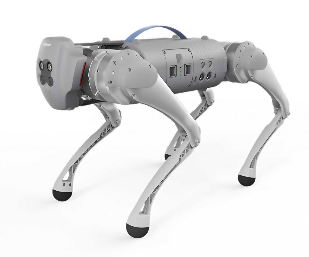
We validated our approach using the Unitree A1 quadruped robot model in Webots. The robot dog was tested on a rugged terrain divided into four regions with varying complexity: Region 1 (flat), Region 2 (moderate slopes), Region 3 (high slopes), and Region 4 (mild slopes). The terrain complexity estimation $C_m[\gamma]$ was recorded during locomotion, as summarized in Table 1.
| Region | $C_m[0]$ (x-direction) | $C_m[1]$ (y-direction) | $C_m[2]$ (z-direction) |
|---|---|---|---|
| Region 1 | 0.0239 | 0.1027 | 0.0064 |
| Region 2 | 0.1129 | 0.1979 | 0.1227 |
| Region 3 | 0.1964 | 0.2688 | 0.1922 |
| Region 4 | 0.0385 | 0.0903 | 0.0239 |
The disturbance compensation forces $F_c$ during motion are shown in Figure 1, illustrating adaptive responses to terrain changes. Comparisons between the original VMC and our enhanced algorithm reveal significant improvements in support force stability, as depicted in Figure 2. The stance phase forces in the $x$, $y$, and $z$ directions exhibit reduced fluctuations, minimizing energy waste and enhancing control.
Gait adjustments are evident in the desired and actual velocity profiles. The original VMC maintains constant desired velocities, leading to large deviations on complex terrain. In contrast, our method modulates desired velocities and gait cycles based on $C_m[\gamma]$, as shown in Figure 3. The step cycle $T_c$ adapts dynamically, with values decreasing in high-complexity regions to improve stability.
Stability was evaluated using the standard deviation of roll angle error ($\text{var}_{\text{roll}}$) and linear momentum error in the $y$-direction ($\text{var}_y$). Our algorithm achieved lower values across all regions, as summarized in Table 2, confirming enhanced stability for the quadruped robot.
| Algorithm | Region 1 $\text{var}_{\text{roll}}$ | Region 1 $\text{var}_y$ | Region 2 $\text{var}_{\text{roll}}$ | Region 2 $\text{var}_y$ | Region 3 $\text{var}_{\text{roll}}$ | Region 3 $\text{var}_y$ | Region 4 $\text{var}_{\text{roll}}$ | Region 4 $\text{var}_y$ |
|---|---|---|---|---|---|---|---|---|
| Original VMC | 0.1267 | 0.2432 | 0.1272 | 0.2759 | 0.1475 | 0.3335 | 0.0812 | 0.1698 |
| ZMP Control | 0.1442 | 0.2773 | 0.1337 | 0.2647 | 0.0933 | 0.2216 | 0.1092 | 0.2309 |
| Our Algorithm | 0.1015 | 0.1898 | 0.0920 | 0.1706 | 0.0816 | 0.1635 | 0.0719 | 0.1371 |
These results demonstrate that our terrain complexity-based control allows the robot dog to actively adapt to unstructured environments, outperforming traditional methods. The quadruped robot maintains smoother velocity tracking and reduced stability metrics, ensuring reliable performance in challenging scenarios.
Conclusion
This paper presents a novel control framework for quadruped robots that integrates online terrain complexity estimation with enhanced virtual model control. By combining foot kinematics and centroid momentum feedback, the robot dog dynamically assesses terrain complexity and adjusts control parameters in both stance and swing phases. Simulation results confirm that our method significantly improves stability on unstructured terrains compared to existing approaches. Future work will focus on real-world deployment, addressing sensor noise, and extending the algorithm for more diverse environments. The adaptability of this approach underscores its potential for advancing quadruped robot applications in complex scenarios.