
In the field of robotics and automation, the ability to accurately measure multi-dimensional forces and moments is crucial for applications such as robotic manipulation, precision assembly, and contour tracking. A six-axis force sensor, capable of detecting three forces (Fx, Fy, Fz) and three moments (Mx, My, Mz) in three-dimensional space, plays a vital role in these domains. However, due to structural design limitations, manufacturing tolerances, and bridge configurations, these sensors often exhibit cross-coupling errors among their output channels, which can significantly degrade measurement accuracy. Static calibration is therefore essential to establish the relationship between applied loads and output signals, enabling decoupling and improving overall performance. This article focuses on the static calibration and performance analysis of a double-E elastomer six-axis force sensor, utilizing experimental data to compute static performance indices and analyze cross-coupling effects through least-squares fitting and slope matrices.
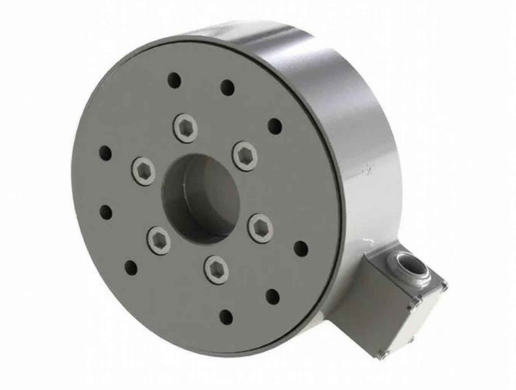
The double-E elastomer six-axis force sensor features a unique elastic body structure designed to enhance sensitivity and stiffness. It consists of an upper E-membrane and a lower E-membrane connected by a central force transmission ring. The upper E-membrane is surrounded by an inner force transmission ring linked to an outer ring via four rectangular beams. The lower E-membrane primarily detects tangential forces (Fx, Fy) and axial force (Fz), while the upper E-membrane measures moments (Mx, My), and the rectangular beams sense the moment around the z-axis (Mz). Strain gauges are attached to the elastic body, forming Wheatstone bridges that convert mechanical strain into voltage signals. These signals are amplified, digitized, and processed to compute the applied forces and moments. The design aims to minimize interference while maintaining high rigidity, making it suitable for direct force measurement in dynamic environments.
The static calibration system for the six-axis force sensor includes a custom-built calibration platform, the sensor unit, a data acquisition card, and a computer running LabVIEW-based data processing software. The calibration platform allows precise application of forces and moments using weighted loads, while the software records six-channel voltage outputs in real-time. The system ensures synchronized data collection and processing, facilitating accurate analysis of sensor behavior under controlled conditions. Calibration is performed by applying incremental loads along each axis, recording outputs during loading and unloading cycles, and repeating the process to ensure reliability. This setup enables comprehensive evaluation of the six-axis force sensor’s static characteristics, including linearity, hysteresis, and repeatability.
The static calibration procedure involves applying forces and moments sequentially along each of the six axes using a weight-based method. For force components (Fx, Fy, Fz), loads are applied in positive and negative directions with uniform increments up to the full-scale range. For example, Fx calibration uses 11 intervals from 0 N to 510 N and back, while Fz calibration covers 13 intervals up to 610 N. Moment components (Mx, My, Mz) are calibrated similarly, with Mx and My using 9 intervals up to 210 N and Mz using 11 intervals up to 260 N. At each load step, voltage outputs from all six channels are recorded during both loading and unloading phases. The process is repeated three times to obtain averaged data, reducing random errors and ensuring consistency. This meticulous approach captures the six-axis force sensor’s response to individual inputs while revealing cross-coupling effects from other axes.
Experimental data from the static calibration of the six-axis force sensor are processed to compute key performance indices, such as nonlinearity, hysteresis, and repeatability errors. For instance, in the Fx direction, the full-scale output (y_F.S.) is calculated as 544.62 mV based on the voltage range. Nonlinearity error (δ_L) is derived from the maximum deviation (Δy_L)_max between the actual output and the least-squares fitted line, expressed as a percentage of y_F.S.:
$$ \delta_L = \frac{(\Delta y_L)_{\text{max}}}{y_{\text{F.S.}}} \times 100\% $$
Hysteresis error (δ_H) accounts for the maximum difference (Δy_H)_max between loading and unloading curves:
$$ \delta_H = \frac{(\Delta y_H)_{\text{max}}}{y_{\text{F.S.}}} \times 100\% $$
Repeatability error (δ_R) is computed using the maximum absolute error (ΔR_max) from multiple cycles:
$$ \delta_R = \frac{\Delta R_{\text{max}}}{y_{\text{F.S.}}} \times 100\% $$
For the Fx direction, these errors are found to be below 0.01%, indicating high precision. Similar calculations are performed for other axes, demonstrating the overall static performance of the six-axis force sensor. The following table summarizes sample data for Fx direction calibration, showing averaged voltage outputs over three cycles:
| Force (N) | Fx-Fx (mV) | Fx-Fy (mV) | Fx-Fz (mV) | Fx-Mx (mV) | Fx-My (mV) | Fx-Mz (mV) |
|---|---|---|---|---|---|---|
| 0 | 2495.37 | 2507.86 | 2546.34 | 2514.80 | 2521.64 | 2534.76 |
| 110 | 2613.50 | 2503.50 | 2550.10 | 2519.37 | 2548.25 | 2520.95 |
| 210 | 2721.07 | 2500.13 | 2553.76 | 2523.09 | 2572.74 | 2507.59 |
| 310 | 2828.31 | 2496.53 | 2558.32 | 2527.58 | 2596.19 | 2495.54 |
| 410 | 2935.00 | 2493.09 | 2563.50 | 2531.52 | 2619.50 | 2482.36 |
| 510 | 3040.70 | 2489.58 | 2568.61 | 2535.73 | 2642.31 | 2470.01 |
Cross-coupling analysis is critical for understanding interactions among the six axes of the six-axis force sensor. By applying least-squares fitting to the calibration data, slope matrices are derived to quantify coupling strengths. For example, when force is applied along Fx, the output voltages from other axes (Fy, Fz, Mx, My, Mz) are analyzed to determine their sensitivity to Fx inputs. The coupling slope for Fx-My is calculated as 0.2141, indicating strong coupling, while slopes for other pairs are below 0.1, representing weak coupling. This analysis is extended to all axes, resulting in a comprehensive slope matrix that defines the six-axis force sensor’s cross-coupling characteristics. The matrix K is expressed as:
$$ K = \begin{bmatrix}
K_{Fx-Fx} & K_{Fx-Fy} & K_{Fx-Fz} & K_{Fx-Mx} & K_{Fx-My} & K_{Fx-Mz} \\
K_{Fy-Fx} & K_{Fy-Fy} & K_{Fy-Fz} & K_{Fy-Mx} & K_{Fy-My} & K_{Fy-Mz} \\
K_{Fz-Fx} & K_{Fz-Fy} & K_{Fz-Fz} & K_{Fz-Mx} & K_{Fz-My} & K_{Fz-Mz} \\
K_{Mx-Fx} & K_{Mx-Fy} & K_{Mx-Fz} & K_{Mx-Mx} & K_{Mx-My} & K_{Mx-Mz} \\
K_{My-Fx} & K_{My-Fy} & K_{My-Fz} & K_{My-Mx} & K_{My-My} & K_{My-Mz} \\
K_{Mz-Fx} & K_{Mz-Fy} & K_{Mz-Fz} & K_{Mz-Mx} & K_{Mz-My} & K_{Mz-Mz}
\end{bmatrix} = \begin{bmatrix}
1.0000 & -0.0352 & 0.0251 & 0.0373 & 0.2141 & -0.0061 \\
0.0390 & 1.0000 & 0.0380 & -0.2150 & 0.0441 & -0.0026 \\
-0.0576 & 0.0235 & 1.0000 & -0.0284 & -0.0397 & 0.0092 \\
-0.0134 & -1.0322 & 0.0412 & 1.0000 & -0.0311 & 0.0041 \\
1.0117 & -0.0144 & 0.0317 & 0.0206 & 1.0000 & 0.0437 \\
0.0045 & -0.0025 & 0.0006 & -0.0054 & 0.0057 & 1.0000
\end{bmatrix} $$
This slope matrix reveals that strong coupling exists between specific pairs, such as Mx-Fy and My-Fx, with slopes exceeding 1.0 or 0.2, respectively. In contrast, Mz shows weak coupling with all other axes, as all related slopes are near zero. The identification of these coupling relationships is fundamental for developing decoupling algorithms to enhance the accuracy of the six-axis force sensor. By applying mathematical techniques like matrix inversion or neural networks, the cross-coupling effects can be compensated, leading to more reliable measurements in practical applications.
In conclusion, the static calibration of the double-E elastomer six-axis force sensor provides valuable insights into its performance and cross-coupling behavior. The experimental results demonstrate low nonlinearity, hysteresis, and repeatability errors, underscoring the sensor’s high static accuracy. However, the presence of significant cross-coupling, particularly between moments and forces, highlights the need for advanced decoupling strategies. Future work will focus on implementing real-time decoupling algorithms to minimize these errors, further improving the six-axis force sensor’s applicability in precision robotics and automation. This study underscores the importance of comprehensive calibration in the development and deployment of multi-axis force sensors, ensuring their reliability in demanding environments.