
The pursuit of lightweight, compact, and high-performance robotic joints has been a central theme in modern robotics, particularly for applications requiring safe physical human-robot interaction (pHRI) and precise force control. Among the various transmission systems, the harmonic drive gear has emerged as a preferred solution due to its exceptional qualities: high torque density, compact size, excellent positional accuracy, and a large, single-stage reduction ratio. However, realizing advanced force-based control paradigms at the joint level necessitates a reliable and accurate method to measure the output torque. While external torque sensors can be added, they increase the joint’s size, weight, and complexity. A more elegant and integrated solution is to embed the sensing capability within the harmonic drive gear itself, leveraging its inherent mechanical compliance. This article presents a comprehensive design, analysis, and experimental validation of a torque sensor embedded within the flexspline of a harmonic drive gear, offering a pathway towards more intelligent and responsive robotic actuators.
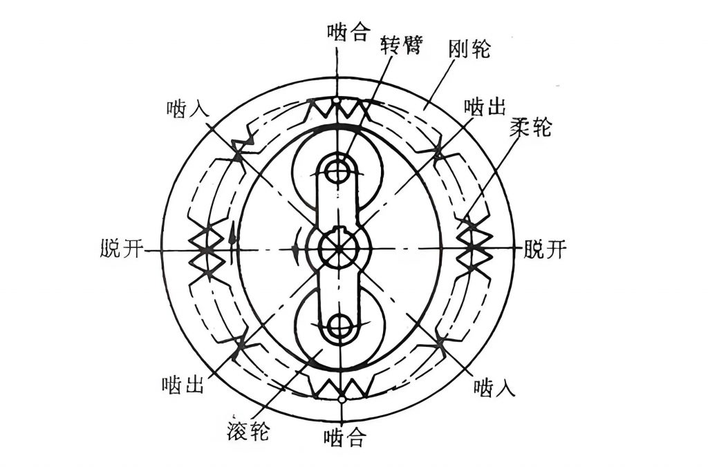
The fundamental operating principle of a harmonic drive gear revolves around the elastic deformation of a flexible component. It consists of three primary elements: the Wave Generator (WG), the Flexspline (FS), and the Circular Spline (CS). The WG, typically comprising an elliptical bearing mounted on an input shaft, is inserted into the FS, a thin-walled, cup-shaped steel component with external teeth on its open end. The CS is a rigid internal gear that meshes with the FS. As the WG rotates, it deforms the FS into an elliptical shape, causing its teeth to engage with the CS teeth at two opposite points. Due to the difference in the number of teeth between the FS and CS, a high reduction ratio is achieved between the input (WG) and output (FS or CS, depending on the configuration). The torque relationship within the system is given by:
$$ T_{wg} = \frac{T_{cs}}{N + 1} = \frac{T_{fs}}{N} $$
where \( T_{wg} \), \( T_{cs} \), and \( T_{fs} \) are the torques on the Wave Generator, Circular Spline, and Flexspline, respectively, and \( N \) is the gear reduction ratio. For a common configuration where the CS is fixed and the FS rotates as the output, the output torque \( T_{out} \) is essentially the negative of \( T_{fs} \). Therefore, accurately measuring the torque experienced by the flexspline provides a direct measurement of the joint’s output torque. The thin-walled diaphragm of the flexspline undergoes torsional deformation proportional to the transmitted torque, making it an ideal location for strain-based sensing.
Our design for the embedded torque sensor focuses on the diaphragm region at the bottom of the flexspline. When torque is transmitted, this diaphragm experiences shear stress. According to the theory of elasticity for thin-walled cylinders under torsion, the shear strain \( \varepsilon_a \) on the surface of the diaphragm can be related to the applied flexspline torque \( T_{fs} \). A simplified model derived from generalized Hooke’s law provides the foundational relationship:
$$ \varepsilon_a = \frac{T_{fs} (r_1 + r_2)}{8\pi a G r_1^2 r_2} $$
Here, \( G \) is the shear modulus of the flexspline material, \( r_1 \) is the radius of the diaphragm’s central hub, \( r_2 \) is the outer radius of the diaphragm, and \( a \) is the diaphragm’s thickness. This equation establishes the principle that strain gauges bonded to this region will experience a resistance change proportional to the joint output torque.
Strain Gauge Configuration and Bridge Circuit Design
The practical implementation involves converting mechanical strain into an electrical signal. We employ metallic foil strain gauges for this purpose. A single gauge is insufficient due to the presence of significant noise. The rotation of the wave generator imposes a cyclical, elliptical deformation on the flexspline, inducing a large, periodic strain interference signal unrelated to the transmitted torque. To reject this common-mode noise, a full Wheatstone bridge configuration with strategically placed gauges is essential.
We propose a configuration using four pairs of strain gauges (\( R_1 \) to \( R_8 \)), arranged symmetrically around the center of the flexspline diaphragm. Each pair consists of two gauges oriented at 90 degrees to each other (forming a “T”-rosette). The four pairs are placed at 0°, 90°, 180°, and 270° positions relative to a reference axis. This symmetrical arrangement is critical. When torque is applied, gauges aligned with the principal tensile stress increase in resistance (\( R_1, R_3, R_5, R_7 \)), while those aligned with the principal compressive stress decrease (\( R_2, R_4, R_6, R_8 \)). The wave generator-induced elliptical deformation affects all gauges in a spatially sinusoidal pattern.
The gauges are wired into a full Wheatstone bridge. The key insight is that the torque-induced strain signals from diametrically opposite and orthogonally oriented gauges add up in the bridge circuit, while the wave generator-induced sinusoidal strain signals, being out of phase for specific gauge pairs, cancel out. For instance, considering one half-bridge, the effective strain is:
$$ (\varepsilon_1 – \varepsilon_2) + (\varepsilon_3 – \varepsilon_4) = [2\varepsilon_a + \psi_0 \sin(2\beta)] + [2\varepsilon_a + \psi_0 \sin(2\beta – \pi)] = 4\varepsilon_a $$
where \( \varepsilon_1, \varepsilon_2, \varepsilon_3, \varepsilon_4 \) are strains at specific gauge locations, and the terms \( \psi_0 \sin(…) \) represent the wave generator interference which cancel out (\( \sin(2\beta – \pi) = -\sin(2\beta) \)). The output voltage \( U_{out} \) of the Wheatstone bridge, when powered by an excitation voltage \( E_{sup} \), becomes:
$$ U_{out} = K \cdot (4\varepsilon_a) \cdot E_{sup} = 4K\varepsilon_a E_{sup} $$
where \( K \) is the gauge factor. Combining this with the strain-torque relation, the sensitivity \( K_R \) of the embedded sensor (before amplification) is derived:
$$ K_R = \frac{U_{out}}{T_{fs}} = \frac{K E_{sup} (r_1 + r_2)}{2\pi a G r_1^2 r_2} $$
The following table summarizes the key design parameters and their influence:
| Parameter | Symbol | Role in Design |
|---|---|---|
| Gauge Factor | \( K \) | Determines electrical output per unit strain. Higher values increase signal level. |
| Diaphragm Thickness | \( a \) | Inversely proportional to sensitivity. Thinner diaphragms yield higher strain but reduce mechanical strength. |
| Material Shear Modulus | \( G \) | Inversely proportional to sensitivity. Lower modulus materials (like certain alloys) increase strain. |
| Hub & Diaphragm Radii | \( r_1, r_2 \) | Geometric parameters set by the harmonic drive gear size. Optimized via finite element analysis. |
| Excitation Voltage | \( E_{sup} \) | Directly proportional to output. Limited by gauge power dissipation and circuit design. |
Precision Placement and Signal Integrity Challenges
The theoretical cancellation of the wave generator interference relies on perfect symmetry and orthogonal placement of the strain gauges. In practice, even minor misalignment during manual bonding introduces positioning errors. These errors prevent complete cancellation, leaving behind a residual periodic noise in the signal, often referred to as “torque ripple.” This ripple is primarily at a frequency related to the gear meshing frequency (approximately twice the motor rotational frequency for a standard harmonic drive gear).
To minimize this error at its source, we developed a precision placement technique using laser marking. First, a Finite Element Analysis (FEA) simulation of the flexspline under load identifies the region of maximum and most uniform strain on the diaphragm. A precise marking pattern, indicating the exact location and orientation for each gauge, is then laser-etched onto the diaphragm surface. This provides a visible, high-accuracy template for bonding, significantly reducing angular and positional errors compared to manual alignment.
Despite this improvement, a small amount of torque ripple inevitably persists due to material imperfections, slight asymmetries in the harmonic drive gear assembly, and non-ideal gauge behavior. This ripple is problematic because its frequency is not fixed; it varies with the motor speed, making simple low-pass filtering ineffective (a fixed cutoff frequency would either attenuate legitimate dynamic torque signals at high speeds or fail to filter ripple at low speeds).
Advanced Signal Processing: Kalman Filtering
To address the time-varying nature of the torque ripple, we employ an adaptive filtering approach based on the Kalman Filter. The Kalman Filter is a recursive algorithm that provides optimal estimates of the state of a dynamic system from a series of noisy measurements. We model the system as follows:
State Equation (Process Model):
The true torque \( T_k \) at time step \( k \) is assumed to evolve with some process noise \( w_k \). A simple random walk model is often sufficient: \( T_k = T_{k-1} + w_k \).
Measurement Equation:
The raw sensor voltage (converted to a torque reading \( z_k \)) is our measurement. It contains the true torque \( T_k \) plus the structured noise (ripple) \( v_k \), which we can model as a sinusoidal component with an estimated frequency \( f_{ripple} \) tied to the known motor speed \( \omega_m \): \( z_k = T_k + A \sin(2\pi f_{ripple} k \Delta t + \phi) + v_k \), where \( A \) and \( \phi \) are amplitude and phase, and \( \Delta t \) is the sampling time. The ripple frequency can be estimated as \( f_{ripple} \approx 2 \cdot (\omega_m / (2\pi N)) \), considering the gear reduction.
The Kalman Filter recursively performs a “predict-update” cycle. It predicts the current state (torque and ripple parameters) based on the previous estimate, then updates this prediction using the new noisy measurement, assigning optimal weights based on the estimated confidence (covariance) in the prediction and the measurement. This effectively learns and subtracts the in-phase ripple component from the signal in real-time, regardless of its frequency. The result is a smoothed torque estimate \( \hat{T}_k \) with dramatically reduced ripple, as shown in comparative plots where peak-to-peak noise is minimized while preserving the actual torque dynamics.
Prototype Testing and Performance Validation
A prototype sensor was implemented on a commercial harmonic drive gear (ratio N=50:1). The test platform consisted of a servo motor driving the wave generator, while the flexspline was fixed. The circular spline served as the output, connected to a calibrated reference torque sensor and a magnetic powder brake to apply variable loads. This configuration protects the strain gauges on the flexspline from rotating electrical contacts (slip rings).
The bridge output was amplified by a factor of 2500. Two sets of experiments were conducted: static (quasi-static) and dynamic.
1. Static Performance:
The motor applied a slowly increasing torque up to 30% of the gear’s rated capacity in 5% increments. The embedded sensor’s reading \( T_{sens} \) was compared against the reference sensor’s reading \( T_{ref} \). The results showed a highly linear relationship but with a consistent offset that grew with torque. This is attributed to load-dependent losses within the harmonic drive gear itself, such as friction and elastic hysteresis in the flexspline wall, which consume a portion of the input torque before it reaches the output. The sensor, measuring strain at the flexspline root, captures the torque at that point, not the final output torque. A linear regression established the conversion: \( T_{ref} = \alpha_s \cdot T_{sens} + \beta_s \).
2. Dynamic Performance:
The motor applied a constant input torque, while the load brake imposed a sinusoidal torque profile on the output. The embedded sensor signal, processed through the Kalman filter, successfully tracked the dynamic reference torque. However, the scaling factor \( \alpha_d \) derived from dynamic data differed from the static factor \( \alpha_s \), due to the influence of speed-dependent effects like viscous damping and dynamic load sharing in the gear teeth. This confirmed the need for separate static and dynamic calibration models.
The performance metrics are summarized below:
| Test Condition | Calibration Model | Maximum Absolute Error | Root Mean Square (RMS) Error | RMS Error (% of Full Scale) |
|---|---|---|---|---|
| Static (Quasi-static ramping) | \( T_{ref} = 1.284T_{sens} – 0.0812 \) | 0.39 Nm | 0.21 Nm | 1.04% |
| Dynamic (Sinusoidal load) | \( T_{ref} = 1.572T_{sens} – 0.0928 \) | 0.64 Nm | 0.265 Nm | 1.27% |
These results demonstrate that the embedded sensor, after appropriate calibration, can estimate the final joint output torque with an accuracy exceeding 98.5% across the tested range, fulfilling the requirements for high-performance joint-level force control.
Torque Conversion and Calibration Philosophy
The relationship between the sensed flexspline torque \( T_{sens} \) and the actual output torque \( T_{ref} \) is not unity and is influenced by multiple factors intrinsic to the harmonic drive gear. We can express this relationship as:
$$ T_{ref} = \eta(T_{sens}, \omega, \dot{\omega}, \theta) \cdot T_{sens} $$
Where \( \eta \) is a dynamic efficiency or torque transfer function that depends on the sensed torque level, output speed \( \omega \), acceleration \( \dot{\omega} \), and angular position \( \theta \). The most significant dependencies are on torque and speed. For many control applications, a piecewise model is effective:
- Static/Low-Speed Model: \( T_{ref} = \alpha_s T_{sens} + \beta_s \). This accounts for constant and load-dependent Coulomb friction.
- Dynamic Model: \( T_{ref} = \alpha_d(\omega) T_{sens} + \beta_d(\omega) \). The coefficients \( \alpha_d \) and \( \beta_d \) can be modeled as functions of speed, potentially linear or identified via lookup tables, to account for viscous losses and changing load distribution.
The calibration process involves collecting \( (T_{sens}, T_{ref}) \) data pairs under various static loads and dynamic trajectories covering the joint’s operational envelope. Polynomial or lookup-table-based fits are then generated. The embedded sensor’s primary role is to provide a high-fidelity, low-noise measurement of \( T_{sens} \), which the joint controller then converts to \( T_{ref} \) using the calibrated model. This decoupling simplifies the sensor design (optimized for clean strain measurement) from the complex, gear-specific loss modeling.
Conclusion
The integration of a torque sensor directly into the flexspline of a harmonic drive gear presents a highly effective solution for enabling force-controlled robotic joints. Our design, utilizing a symmetrical eight-gauge full-bridge configuration, laser-marking for precision placement, and Kalman filtering for adaptive noise rejection, successfully addresses the key challenges of interference rejection and signal integrity. Experimental validation confirms that the proposed sensor can achieve static and dynamic torque measurement accuracy better than 1.3% of full scale after a straightforward calibration that accounts for the harmonic drive gear‘s internal losses. This approach minimizes the impact on the joint’s size and weight, preserves the original compliance of the gear for safety, and provides the critical joint-level force feedback needed for advanced impedance and admittance control strategies. As robotics continues to advance towards more collaborative and dynamic applications, such deeply embedded sensing technologies will be fundamental in creating the next generation of intelligent and responsive actuators.