
The integration of robotic technology into the textile and apparel industry represents a significant leap towards automation and intelligent manufacturing. While robots have permeated various stages of textile processing, the automated handling of soft, compliant, and irregularly stacked fabrics remains a formidable challenge. This difficulty primarily stems from the inherent properties of fabrics—their flexibility, deformability, and unpredictable resting states—which impose stringent requirements on a robot’s end-effector. Conventional grippers, designed for rigid objects, often fail to achieve stable and precise grasps on such malleable materials without causing damage or slippage.
In this context, the dexterous robotic hand emerges as a pivotal solution. Mimicking the anatomical structure and functional capabilities of the human hand, a multi-fingered dexterous robotic hand offers unparalleled adaptability. Its multiple degrees of freedom (DoFs) allow for complex, finger-gaiting motions and the ability to conform to a wide variety of object shapes, making it ideally suited for the delicate task of fabric manipulation. The core of enabling a dexterous robotic hand to perform a successful grasp lies not only in its mechanical design but also in sophisticated motion planning. Trajectory planning dictates the precise path each finger follows from an initial position to the final grasp points on the fabric. A well-planned trajectory ensures a smooth, collision-free approach, stable contact establishment, and ultimately, a reliable grip. Poor planning can lead to missed grasps, fabric displacement, or unstable prehension. Therefore, this paper focuses on the design and, more critically, the motion trajectory planning for a three-fingered dexterous robotic hand specifically tasked with grasping soft fabric. We propose a hybrid planning strategy combining joint-space and Cartesian-space methods to guarantee accuracy, stability, and computational efficiency throughout the grasping operation.
1. Design and Kinematic Modeling of the Dexterous Robotic Hand
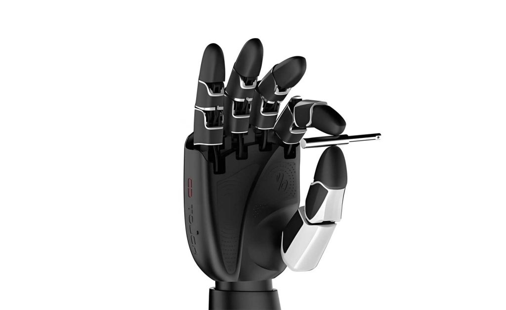
The design of the end-effector is the first critical step. For grasping deformable objects like fabric, the number of fingers and their DoF configuration are paramount. A two-fingered gripper, while simple, often lacks the stability margin required for secure grasping of limp materials. Conversely, a hand with more than three fingers introduces mechanical complexity, control redundancy, and increased difficulty in coordination without necessarily providing proportional benefits for this specific task. Consequently, a three-fingered architecture is chosen as an optimal balance between simplicity, controllability, and grasp stability.
Each finger of the dexterous robotic hand must possess sufficient dexterity to reach desired points in the workspace from various orientations. To this end, each finger is designed with 4 rotational DoFs. The first joint axis is oriented perpendicularly to the subsequent three, which are parallel, resembling a simplified human finger structure with abduction/adduction at the base and flexion/extension in the remaining links. This configuration provides a good compromise between workspace volume and mechanical complexity. The kinematic chain for a single finger is illustrated in the following Denavit-Hartenberg (D-H) parameter table, which systematically defines the spatial relationship between consecutive links.
| Link i | αi-1 (rad) | ai-1 (mm) | di (mm) | θi (rad) |
|---|---|---|---|---|
| 1 | 0 | L1 | 0 | θ1 |
| 2 | 0 | L2 | 0 | θ2 |
| 3 | 0 | L3 | 0 | θ3 |
| 4 | 0 | L4 | 0 | θ4 |
The homogeneous transformation matrix between link i-1 and link i is given by the standard D-H formulation:
$$^{i-1}\mathbf{T}_i = \begin{bmatrix}
\cos\theta_i & -\sin\theta_i \cos\alpha_{i-1} & \sin\theta_i \sin\alpha_{i-1} & a_{i-1}\cos\theta_i\\
\sin\theta_i & \cos\theta_i \cos\alpha_{i-1} & -\cos\theta_i \sin\alpha_{i-1} & a_{i-1}\sin\theta_i\\
0 & \sin\alpha_{i-1} & \cos\alpha_{i-1} & d_i\\
0 & 0 & 0 & 1
\end{bmatrix}$$
Given the parameters in the table (where all αi-1 = 0), the transformation matrices simplify. The complete forward kinematics for the fingertip position relative to the finger’s base frame is obtained by the chain multiplication:
$$^{0}\mathbf{T}_4 = ^{0}\mathbf{T}_1 \cdot ^{1}\mathbf{T}_2 \cdot ^{2}\mathbf{T}_3 \cdot ^{3}\mathbf{T}_4$$
Substituting the simplified D-H matrices yields the fingertip pose matrix:
$$^{0}\mathbf{T}_4 = \begin{bmatrix}
c_{1234} & -s_{1234} & 0 & L_1c_1 + L_2c_{12} + L_3c_{123} + L_4c_{1234}\\
s_{1234} & c_{1234} & 0 & L_1s_1 + L_2s_{12} + L_3s_{123} + L_4s_{1234}\\
0 & 0 & 1 & 0\\
0 & 0 & 0 & 1
\end{bmatrix}$$
where $c_1 = \cos\theta_1$, $s_1 = \sin\theta_1$, $c_{12} = \cos(\theta_1+\theta_2)$, $s_{12} = \sin(\theta_1+\theta_2)$, and so on. The last column vector $[P_x, P_y, 0, 1]^T$ defines the Cartesian coordinates $(x, y)$ of the fingertip in the base plane (assuming planar motion for this model), which is crucial for subsequent trajectory planning. Establishing this kinematic model is fundamental for both planning the path of the dexterous robotic hand and for solving the inverse kinematics needed to determine joint angles from desired Cartesian positions.
2. Analysis of the Grasping Motion Process
Executing a fabric grasp with a dexterous robotic hand is a sequential process that must be carefully choreographed. The motion can be logically divided into two primary phases: the approach phase and the pre-grasp/contact phase. Each phase has distinct requirements that inform the choice of trajectory planning domain.
During the approach phase, the fingers move from their initial, possibly folded or parked, configuration to a “preshape” or “approach” posture near the intended fabric grasp points. In this phase, the primary objectives are to avoid collisions (with the environment, the fabric, or between fingers) and to move efficiently. The exact Cartesian path of the fingertips is not critically constrained as long as they reach the vicinity of the target. This makes joint-space planning highly suitable. Planning directly in the joint angle space is computationally efficient because it avoids the need for continuous inverse kinematics solutions. One can simply define smooth functions for each joint angle over time, ensuring the fingers move synchronously to their approach postures.
The pre-grasp/contact phase begins once the fingers are near the fabric and ends when stable contact is established at the predefined grasp points. This phase is critical for success. The fingertips must now follow very specific, straight-line paths in Cartesian space to ensure they contact the fabric at the exact intended points simultaneously. A non-straight path or unsynchronized arrival could brush against the fabric, displacing it, or result in an uneven initial contact that compromises the grasp stability. Furthermore, the velocity profile upon contact is important to apply the appropriate initial contact force. Therefore, this phase is best handled in Cartesian-space planning, where the desired straight-line path of each fingertip is explicitly defined, and the corresponding joint trajectories are computed via inverse kinematics.
This two-phase strategy—joint-space planning for the gross approach and Cartesian-space planning for the final precise approach—forms the hybrid planning framework for the dexterous robotic hand. It leverages the strengths of each method: the computational simplicity of joint-space planning for the long, unconstrained travel and the path accuracy of Cartesian-space planning for the critical final segment.
3. Trajectory Planning Algorithms
To implement the hybrid planning strategy, specific algorithms are selected for each phase to meet the requirements of smoothness, boundary condition compliance, and computational tractability.
3.1 Quintic Polynomial Planning in Joint Space
For the joint-space approach phase, a fifth-order (quintic) polynomial is chosen to define the joint trajectory $\theta(t)$. A quintic polynomial allows the specification of constraints not only on initial and final position but also on velocity and acceleration. This is essential for ensuring the dexterous robotic hand starts and ends the approach phase smoothly, with zero velocity and zero acceleration, preventing sudden jerks that could induce vibrations or overshoot.
The general form of the quintic polynomial for a single joint is:
$$\theta(t) = a_0 + a_1 t + a_2 t^2 + a_3 t^3 + a_4 t^4 + a_5 t^5$$
where $t$ is time, normalized from $0$ to the movement duration $t_d$. The constraints for the approach phase are typically:
$$\theta(0) = \theta_0, \quad \dot{\theta}(0) = 0, \quad \ddot{\theta}(0) = 0$$
$$\theta(t_d) = \theta_d, \quad \dot{\theta}(t_d) = 0, \quad \ddot{\theta}(t_d) = 0$$
Here, $\theta_0$ and $\theta_d$ are the initial and desired (approach) joint angles, respectively. Solving for the coefficients $a_i$ using these six boundary conditions yields:
$$\begin{aligned}
a_0 &= \theta_0 \\
a_1 &= 0 \\
a_2 &= 0 \\
a_3 &= \frac{10(\theta_d – \theta_0)}{t_d^3} \\
a_4 &= -\frac{15(\theta_d – \theta_0)}{t_d^4} \\
a_5 &= \frac{6(\theta_d – \theta_0)}{t_d^5}
\end{aligned}$$
Substituting these back gives the complete joint trajectory equation:
$$\theta(t) = \theta_0 + \frac{10(\theta_d – \theta_0)}{t_d^3} t^3 – \frac{15(\theta_d – \theta_0)}{t_d^4} t^4 + \frac{6(\theta_d – \theta_0)}{t_d^5} t^5$$
The corresponding velocity and acceleration profiles, obtained by differentiation, are:
$$\dot{\theta}(t) = \frac{30(\theta_d – \theta_0)}{t_d^3} t^2 – \frac{60(\theta_d – \theta_0)}{t_d^4} t^3 + \frac{30(\theta_d – \theta_0)}{t_d^5} t^4$$
$$\ddot{\theta}(t) = \frac{60(\theta_d – \theta_0)}{t_d^3} t – \frac{180(\theta_d – \theta_0)}{t_d^4} t^2 + \frac{120(\theta_d – \theta_0)}{t_d^5} t^3$$
These profiles are smooth and continuous, ensuring stable motion for every joint of the dexterous robotic hand during the approach.
3.2 Spatial Linear Interpolation with Parabolic Blends in Cartesian Space
For the final precise approach in Cartesian space, linear interpolation is the most straightforward method to generate a straight-line path between the approach point $\mathbf{P}_a = (x_a, y_a, z_a)$ and the final grasp point $\mathbf{P}_g = (x_g, y_g, z_g)$. The position of an interpolated point at any given normalized time $\lambda$ (where $\lambda = 0$ at $\mathbf{P}_a$ and $\lambda = 1$ at $\mathbf{P}_g$) is:
$$\mathbf{P}(\lambda) = \mathbf{P}_a + \lambda (\mathbf{P}_g – \mathbf{P}_a) = \mathbf{P}_a + \lambda \Delta\mathbf{P}$$
However, pure linear interpolation in time (i.e., $\lambda = t/t_d$) results in a discontinuous velocity at the path endpoints (a sudden start and stop). To achieve smooth motion, a linear segment with parabolic blends (LSPB) is employed. This method replaces the corners of the velocity profile with parabolic arcs, resulting in constant acceleration/deceleration periods.
| Parameter | Description | Formula |
|---|---|---|
| $L$ | Total path length | $L = \|\mathbf{P}_g – \mathbf{P}_a\|$ |
| $v$ | Cruising velocity (during linear segment) | Design choice |
| $a$ | Acceleration/deceleration magnitude | Design choice ($a > 0$) |
| $t_b$ | Duration of one blend (parabolic) segment | $t_b = v / a$ |
| $L_b$ | Distance covered during one blend segment | $L_b = \frac{1}{2} a t_b^2 = v^2 / (2a)$ |
| $T$ | Total trajectory time | $T = \frac{L}{v} + \frac{v}{a}$ (if $L \ge 2L_b$) |
The condition $L \ge 2L_b$ ensures there is a linear (constant velocity) segment between the two parabolic blends. The normalized time parameter $\lambda(t)$ is now no longer a simple linear function of time. For a trajectory normalized to total time $T=1$, and with normalized blend time $t_{b\lambda} = t_b/T$, the function $\lambda(\tau)$ (where $\tau = t/T$) is piecewise:
$$
\lambda(\tau) =
\begin{cases}
\frac{1}{2} a_\lambda \tau^2, & 0 \leq \tau \leq t_{b\lambda} \\
a_\lambda t_{b\lambda} (\tau – \frac{t_{b\lambda}}{2}), & t_{b\lambda} < \tau \leq 1 – t_{b\lambda} \\
1 – \frac{1}{2} a_\lambda (1 – \tau)^2, & 1 – t_{b\lambda} < \tau \leq 1
\end{cases}
$$
where $a_\lambda = 1 / (t_{b\lambda}(1 – t_{b\lambda}))$ is the normalized acceleration. This $\lambda(\tau)$ function is continuous and has continuous first derivatives (velocity), providing the smooth motion required for the dexterous robotic hand to make precise, stable contact with the fabric.
4. Simulation and Experimental Verification
The proposed three-fingered dexterous robotic hand design and the hybrid trajectory planning algorithm were validated through simulation using the MATLAB environment, specifically leveraging the Robotics Toolbox for kinematic modeling and visualization. The simulation process followed these steps:
1. Model Instantiation: The D-H parameters were used to create serial-link models for each of the three fingers. Initial joint configurations were set to define a “home” position for the hand.
2. Point Definition: Key points for the trajectory were defined:
- Start Point (S): The initial folded configuration of the hand.
- Approach Point (A): A pre-grasp posture where fingers are positioned near the intended fabric grasp locations but not in contact. Joint angles $\theta_d$ for this point were calculated via inverse kinematics from desired Cartesian positions.
- Grasp Point (G): The final points on the fabric surface where fingertip contact is desired. Corresponding joint angles $\theta_g$ were also computed.
3. Trajectory Generation:
- Segment S-A (Joint Space): For each joint of each finger, a quintic polynomial trajectory was generated using the equations from Section 3.1, with boundary conditions $\theta_0$, $\theta_d$, and zero start/end velocity/acceleration.
- Segment A-G (Cartesian Space): For each fingertip, a straight-line path was defined between its position at point A and point G. The LSPB algorithm (Section 3.2) was used to generate a sequence of Cartesian points along this line. Inverse kinematics was then solved at each intermediate point to obtain the corresponding joint angle trajectory.
4. Results and Analysis: The simulation produced the following key outputs, confirming the efficacy of the planning method for the dexterous robotic hand:
| Plot/Output | Description | Observations & Implications |
|---|---|---|
| 3D Hand Model Animation | Visualization of the hand moving through the complete S-A-G trajectory. | Confirmed that all fingers moved synchronously and reached their target grasp points accurately without collision. The motion appeared smooth and natural. |
| Joint Angle Trajectories | Plots of $\theta_i(t)$ for all joints across all fingers. | All curves were smooth, continuous, and passed exactly through the specified via-points (S, A, G). The transition at point A between the quintic polynomial (S-A) and the IK-derived (A-G) trajectory was seamless. |
| Joint Velocity & Acceleration Profiles | Plots of $\dot{\theta}_i(t)$ and $\ddot{\theta}_i(t)$. | Velocity profiles started and ended at zero. Acceleration profiles were finite and continuous. This verifies the absence of impulsive forces, ensuring stable and vibration-free motion of the dexterous robotic hand mechanism. |
| Fingertip Cartesian Trajectories | Plot of the $(x, y, z)$ path of each fingertip in space. | Clearly showed a smooth curve from S to A (path not strictly constrained), followed by a perfect straight line from A to G. This visually validates the hybrid planning approach: free-form approach followed by precise linear approach. |
The simulation results conclusively demonstrate that the proposed hybrid trajectory planning framework successfully guides the three-fingered dexterous robotic hand from its initial state to a precise fabric grasp configuration. The quintic polynomial in joint space ensures a smooth, efficient approach, while the Cartesian linear interpolation with parabolic blends guarantees accurate, synchronized, and stable contact establishment—a critical requirement for handling soft, displaceable fabrics.
5. Conclusion
This paper addressed the specialized problem of trajectory planning for a multi-fingered dexterous robotic hand tasked with grasping soft fabric. The challenge lies in managing the fabric’s compliance and unpredictability, which demands a highly adaptable and precisely controlled end-effector. The solution presented involves a systematic two-phase strategy. First, a three-fingered dexterous robotic hand with four DoFs per finger was designed and its kinematics modeled using the D-H convention, providing the foundation for all motion planning calculations.
The core contribution is the hybrid trajectory planning methodology. The approach phase utilizes quintic polynomial interpolation in joint space. This method is computationally efficient and provides direct control over joint-level smoothness by enforcing zero boundary conditions on velocity and acceleration, ensuring the hand moves stably to the vicinity of the target. The critical pre-grasp phase employs spatial linear interpolation with parabolic blends in Cartesian space. This guarantees that each fingertip follows an exact straight-line path to its designated contact point on the fabric, with a smooth velocity profile that prevents sudden impacts or fabric displacement. The seamless integration of these two methods leverages their respective strengths.
Comprehensive simulation in MATLAB using the Robotics Toolbox validated the entire approach. The results showed smooth, continuous, and accurate joint and Cartesian trajectories. All fingers of the dexterous robotic hand synchronized correctly and reached their final grasp points as planned, confirming the practical viability of the algorithm. This work provides a solid theoretical and algorithmic foundation for implementing intelligent, sensor-driven fabric handling robots in the textile and apparel industry, moving closer to fully automated flexible material manipulation.