
In the realm of advanced manufacturing, robotics has emerged as an indispensable tool, often serving as a benchmark for a nation’s industrial and technological prowess. Among the critical components that enable high-precision robotic motion, the Rotary Vector (RV) reducer stands out due to its exceptional load capacity, compact design, and high transmission accuracy. However, the performance of an RV reducer is highly sensitive to manufacturing imperfections, particularly tooth profile errors in its cycloidal gear set. These errors, arising from limitations in machine tool accuracy, cutter precision, fixture alignment, and gear blank quality, can significantly degrade transmission precision, leading to uneven load distribution, stress concentration, and reduced operational lifespan. Therefore, a thorough investigation into the influence of tooth profile errors on the meshing characteristics and transmission error of the cycloidal-pin gear pair is paramount for designing and manufacturing high-performance RV reducers.
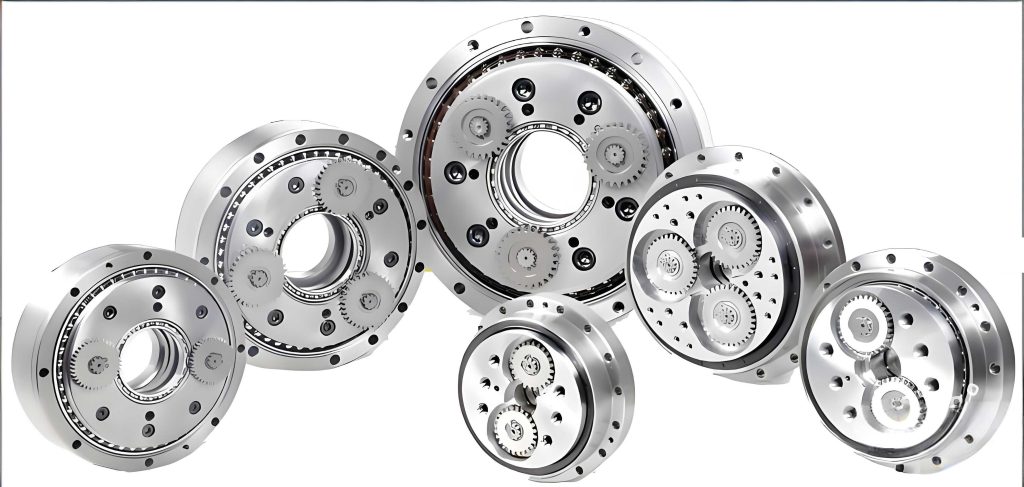
Previous research has laid a foundation for understanding error sensitivities in RV reducers. Studies have focused on error analysis, dynamic modeling considering various manufacturing and assembly errors, and methods for calculating meshing backlash. Notably, the application of Tooth Contact Analysis (TCA) to actual tooth surfaces incorporating measured profile errors remains relatively unexplored. This work aims to address this gap by developing a methodology to assess the impact of real-world tooth profile errors on the transmission error of an RV reducer’s cycloidal stage. The core approach involves acquiring measured tooth profile data, reconstructing the actual tooth flank using a Non-Uniform Rational B-Spline (NURBS) representation, and performing a digital tooth contact analysis based on gear meshing theory to obtain the transmission error curve.
The initial step in this analysis involves obtaining a digital representation of the actual cycloidal gear tooth flank. In practical manufacturing, the produced gear deviates from its theoretical design. These deviations, or tooth profile errors, are typically measured using specialized gear measuring equipment. For this study, we consider measurement data collected at discrete points along the tooth profile. To ensure a representative analysis, the measurement points are selected at equal intervals of the meshing phase angle, providing a uniform distribution across the active tooth flank. The theoretical tooth profile of a cycloidal gear, often modified with parabolic corrections for improved performance, serves as the reference. For a gear with parabolic modification, the theoretical flank can be described in its transverse plane. The homogeneous coordinate form of the theoretical tooth profile equation is given by:
$$ \mathbf{r_c}(\varphi) = [x_c(\varphi), y_c(\varphi), 0, 1]^T $$
where $\varphi$ is the generating angle or mesh phase angle parameter. The corresponding unit normal vector at any point on this theoretical profile is:
$$ \mathbf{n_c}(\varphi) = [n_{xc}(\varphi), n_{yc}(\varphi), 0]^T $$
Let $\delta’_{\varphi_i}$ represent the measured tooth profile error at the i-th measurement point, taken along the normal direction of the theoretical profile at that specific meshing phase angle $\varphi_i$. The coordinates of the actual tooth surface point $(X_c, Y_c)$ can then be calculated by superimposing this error onto the theoretical point:
$$
\begin{cases}
X_c = x_c(\varphi_i) + n_{xc}(\varphi_i) \cdot \delta’_{\varphi_i} \\
Y_c = y_c(\varphi_i) + n_{yc}(\varphi_i) \cdot \delta’_{\varphi_i}
\end{cases}
$$
This process yields a set of discrete coordinate points $(X_c, Y_c)$ that represent the actual, error-containing tooth flank. A typical distribution of such measurement points is visualized conceptually, showing points spaced evenly along the tooth curve from the root to the tip region.
The discrete data points must be converted into a continuous mathematical representation suitable for further contact analysis. This is achieved through curve fitting. The Non-Uniform Rational B-Spline (NURBS) curve is an excellent tool for this purpose due to its flexibility, precision, and ability to represent complex shapes with a compact set of control points. A NURBS curve of degree p is defined as:
$$ \mathbf{C}(u) = \frac{\sum_{i=0}^{n} N_{i,p}(u) w_i \mathbf{P}_i}{\sum_{i=0}^{n} N_{i,p}(u) w_i} $$
where $\mathbf{P}_i$ are the control points, $w_i$ are the corresponding weights, $N_{i,p}(u)$ are the p-th degree B-spline basis functions defined on a non-uniform knot vector $U$, and $u$ is the curve parameter. For fitting a cubic (degree 3) curve to our measured data, we can simplify the process by considering a non-rational B-spline if weights are not crucial for the fit. The vector function for a cubic B-spline curve is:
$$ \mathbf{p}(u) = \sum_{i=0}^{n} \mathbf{d}_i N_{i,3}(u) $$
Here, $\mathbf{d}_i$ ($i = 0, 1, …, n$) are the control vertices, and $n+1$ is the number of control points. The basis functions $N_{i,3}(u)$ are defined recursively using the Cox-de Boor algorithm. The fitting process involves determining the control point vector $\mathbf{d}_i$ that minimizes the deviation between the fitted curve and the measured data points. This is typically done through an interpolation or least-squares approximation algorithm. Once the control points are computed, the equation above provides a continuous, analytical expression $\mathbf{R_c}(u)$ for the digitized tooth profile, encapsulating the measured tooth profile errors. The accuracy of this NURBS fitting is critical. To validate it, a separate set of points from the theoretical profile can be fitted, and the deviation between the NURBS-reconstructed theoretical curve and the original theoretical equation at various test points is computed. The fitting error should be orders of magnitude smaller than the tooth profile errors themselves to ensure the digitized flank faithfully represents the actual geometry.
With the digitized tooth flank of the cycloidal gear available as $\mathbf{R_c}(u)$, we proceed to the Tooth Contact Analysis (TCA) for the cycloidal-pin gear pair. TCA is a numerical simulation technique used to determine the transmission error and contact patterns under loaded or unloaded conditions. For this analysis, we consider the unloaded kinematic transmission error. The fundamental principle is to establish the mathematical condition for continuous contact between the mating tooth flanks. We define coordinate systems attached to the cycloidal gear ($S_c$), the pin gear ($S_p$), and a fixed frame ($S_f$). The pin gear is typically considered stationary in the RV reducer’s second stage, but for TCA, we often let one component rotate. The transformation matrices between these systems incorporate the gear geometry and rotational displacements.
The surface of the cycloidal gear in its own coordinate system $S_c$ is $\mathbf{r}^{(c)}(u) = [x_c(u), y_c(u), 0]^T$. The surface of a pin (modeled as a circle) in the pin gear coordinate system $S_p$ is $\mathbf{r}^{(p)}(\beta) = [0, -r_{rp}\cos\beta, r_{rp}\sin\beta]^T$, where $r_{rp}$ is the pin radius and $\beta$ is an angular parameter locating a point on the pin circle. The pin gear coordinate system is fixed, and the cycloidal gear rotates. Alternatively, to find contact points sequentially, we can consider the pin gear rotating and the cycloidal gear responding. Through coordinate transformations, both surfaces are expressed in the fixed coordinate system $S_f$. The condition for contact at any instant is that a point on the cycloidal gear coincides with a point on the pin surface, and their unit normals are collinear (opposite in direction). This yields a system of equations:
$$
\begin{cases}
\mathbf{r}_f^{(c)}(u, \phi_2) = \mathbf{r}_f^{(p)}(\beta, \phi_1) \\
\mathbf{n}_f^{(c)}(u, \phi_2) = -\mathbf{n}_f^{(p)}(\beta, \phi_1)
\end{cases}
$$
Here, $\phi_1$ represents the rotation angle of the pin gear (or input), and $\phi_2$ represents the rotation angle of the cycloidal gear (or output). In a more common formulation for a fixed pin gear and rotating cycloidal gear, $\phi_1$ might be set to zero, and the cycloidal gear’s rotation is the input. However, to compute transmission error, we consider the kinematic relationship. The system above consists of three independent scalar equations (from the vector equality of positions and the collinearity of normals, which gives two independent conditions) with four unknowns: $u$, $\beta$, $\phi_1$, and $\phi_2$. By choosing one parameter as the input, typically the pin gear rotation $\phi_1$, the system can be solved numerically for the remaining three unknowns $u$, $\beta$, and $\phi_2$ for each contact position. This process is repeated for a full cycle of engagement to map out the contact path and the corresponding output rotation $\phi_2$ for each input step $\phi_1$.
The transmission error (TE) is then defined as the deviation of the actual output position from the position expected under ideal, conjugate motion. For a cycloidal-pin pair with $z_c$ cycloidal teeth and $z_p$ pins, the ideal kinematic relationship is $\phi_2 = (z_p / z_c) \phi_1$. The transmission error $\Delta E$ is thus:
$$ \Delta E(\phi_1) = \left( \phi_2(\phi_1) – \phi_{20} \right) – \frac{z_p}{z_c} \left( \phi_1 – \phi_{10} \right) $$
where $(\phi_{10}, \phi_{20})$ is a reference pair of angles at a chosen initial contact point. Often, $\Delta E$ is expressed in arc-minutes or arc-seconds for high-precision applications like RV reducers. This TE curve, plotted over one mesh cycle, reveals the kinematic performance. A perfectly conjugate gear pair would yield $\Delta E = 0$. However, due to modifications and errors, the TE curve is non-zero and its characteristics—amplitude, shape, and frequency content—directly impact noise, vibration, and smoothness of operation.
To illustrate the methodology and quantify the impact of tooth profile errors, we present a detailed case study based on a specific RV reducer model. The basic geometric parameters of the cycloidal gear set are summarized in the table below. These parameters define the theoretical design, including modification values used to optimize load distribution and reduce backlash.
| Parameter | Symbol | Value |
|---|---|---|
| Number of Cycloidal Gear Teeth | $z_c$ | 11 |
| Number of Pin Gear Teeth (Pins) | $z_p$ | 12 |
| Pin Radius | $r_{rp}$ | 7.0 mm |
| Eccentricity | $a$ | 4.0 mm |
| Pin Center Distribution Circle Radius | $r_p$ | 90.0 mm |
| equidistant Modification Amount | $\Delta r_{rp}$ | +0.01 mm |
| Profile Shift Modification Amount | $\Delta r_{p}$ | -0.02 mm |
For this RV reducer, a physical cycloidal gear was measured using a precision gear measuring machine. The tooth profile error was recorded at 90 distinct points along one tooth flank, spaced at equal meshing phase angles. The measured error values (in micrometers) for a single tooth are tabulated below. This data represents a realistic error profile that might result from a manufacturing process.
| Point Index | Error (µm) | Point Index | Error (µm) | Point Index | Error (µm) | Point Index | Error (µm) |
|---|---|---|---|---|---|---|---|
| 1 | 0.1 | 24 | 4.0 | 47 | -0.4 | 70 | 2.6 |
| 2 | 0.3 | 25 | 2.9 | 48 | -0.9 | 71 | 2.3 |
| 3 | 0.7 | 26 | 2.6 | 49 | 0.2 | 72 | 2.4 |
| 4 | 1.7 | 27 | 2.7 | 50 | -0.1 | 73 | 2.7 |
| 5 | 2.7 | 28 | 1.8 | 51 | 0.1 | 74 | 2.8 |
| 6 | 3.7 | 29 | 1.6 | 52 | 0.3 | 75 | 3.3 |
| 7 | 4.8 | 30 | 1.0 | 53 | 0.5 | 76 | 3.8 |
| 8 | 5.8 | 31 | 1.3 | 54 | 0.7 | 77 | 3.6 |
| 9 | 6.6 | 32 | 0.9 | 55 | 1.2 | 78 | 3.4 |
| 10 | 6.8 | 34 | 0.5 | 56 | 1.4 | 79 | 3.2 |
| 11 | 7.2 | 35 | 0.1 | 57 | 1.5 | 80 | 2.7 |
| 12 | 7.7 | 36 | -0.2 | 58 | 1.7 | 81 | 3.1 |
| 13 | 8.3 | 37 | -0.1 | 59 | 1.9 | 82 | 3.8 |
| 14 | 5.8 | 38 | -0.7 | 60 | 2.1 | 83 | 3.4 |
| 15 | 8.2 | 39 | -0.5 | 61 | 3.2 | 84 | 2.5 |
| 16 | 8.2 | 40 | -0.1 | 62 | 3.6 | 85 | 1.7 |
| 17 | 7.2 | 41 | -0.3 | 63 | 3.9 | 86 | 1.8 |
| 18 | 7.2 | 42 | -0.6 | 64 | 4.3 | 87 | 1.2 |
| 19 | 7.6 | 43 | -0.7 | 65 | 3.5 | 88 | 0.5 |
| 20 | 6.7 | 44 | -0.8 | 66 | 3.3 | 89 | 0.1 |
| 21 | 5.7 | 45 | -0.5 | 67 | 3.4 | 90 | -0.1 |
| 22 | 4.8 | 46 | -0.2 | 68 | 3.2 | ||
| 23 | 4.6 | 69 | 3.2 |
Using the method described earlier, these error values are superimposed onto the theoretical flank points according to Equation (3) to generate 90 actual surface data points. A cubic NURBS curve is then fitted to this data set. The fitting process involves calculating the knot vector and control points that best approximate the data. The resulting digitized flank $\mathbf{R_c}(u)$ is a smooth curve that incorporates all the measured imperfections. To ensure the fidelity of this digital model, a validation step is performed. A NURBS curve is fitted to 90 points sampled directly from the theoretical profile equation. Then, at 37 different, independently chosen meshing phase angles, the normal distance between the NURBS-fitted theoretical curve and the exact theoretical profile is computed. These fitting errors were found to be on the order of $1 \times 10^{-8}$ mm, which is negligible compared to the micron-level tooth profile errors. This confirms that the NURBS representation is an accurate substitute for the actual geometry for the purpose of TCA.
Next, the TCA procedure is implemented. A computer program is developed to solve the system of contact equations numerically. For a sequence of input pin gear rotation angles $\phi_1$ spanning one mesh cycle (involving multiple teeth due to the multi-tooth contact nature of cycloidal drives), the program finds the corresponding cycloidal gear rotation $\phi_2$ and contact point parameters $u$ and $\beta$ that satisfy the contact conditions. The transmission error $\Delta E$ is then computed using Equation (6). This analysis is performed twice: first for the ideal, theoretical tooth profile (without errors), and second for the digitized profile containing the measured errors.
The results are presented as transmission error curves. For the theoretical profile with parabolic modifications but no random errors, the transmission error curve is typically a smooth, parabolic-like shape. This shape is a direct consequence of the intentional profile modifications designed to pre-compensate for elastic deflections under load and to ensure proper meshing. The curve for our example RV reducer, calculated via TCA, exhibits a single, broad peak or trough depending on the modification signs, with a relatively flat region near the extreme value. The amplitude of this theoretical transmission error is within a few arc-seconds, reflecting the high kinematic accuracy possible with precise manufacturing.
In stark contrast, the transmission error curve obtained when the measured tooth profile errors are incorporated shows significant distortion. The smooth parabolic shape is disrupted, replaced by a wavy, oscillatory pattern. The curve often displays multiple local maxima and minima within a single mesh cycle. The amplitude of the transmission error fluctuations is generally larger than that of the theoretical curve. More importantly, the pattern is not symmetrical or predictable based on design alone; it directly mirrors the spatial distribution of the manufacturing errors along the tooth flank. Peaks in the error curve correspond to regions on the tooth where positive or negative profile errors disrupt the conjugate motion most severely. The crossing points of the error curve (where it passes through zero) may not be evenly spaced, indicating uneven load sharing among simultaneously contacting tooth pairs. This has profound implications for the dynamic performance of the RV reducer. The high-frequency components introduced by the wavy TE curve can excite torsional vibrations, leading to increased noise and potential resonance issues. Furthermore, the increased peak-to-peak amplitude of the TE directly translates to a degradation in the positioning accuracy of the robotic joint driven by the RV reducer.
The sensitivity of the RV reducer’s performance to these errors underscores the importance of tight manufacturing tolerances. Even sub-micron level errors, when integrated over the entire tooth profile, can cause arc-second level changes in transmission error, which is critical for applications requiring precision below one arc-minute. This analysis provides a quantitative tool for quality control. By establishing a relationship between measured tooth profile error maps and the resulting transmission error, manufacturers can set acceptance limits on profile errors not just based on simple maximum deviation, but on the predicted impact on kinematic performance. For instance, certain error profiles (like a consistent slope) might be more detrimental than others (like high-frequency roughness).
Extending this work, the digitized tooth flank model can be seamlessly integrated into more advanced simulations. For loaded Tooth Contact Analysis (LTCA), the same geometric model is used, but elastic deformations of the teeth, bearings, and housing are considered to compute contact stresses, load distribution, and static transmission error under torque. The presence of profile errors will significantly alter the load distribution, potentially leading to stress concentrations on certain teeth that carry disproportionate load. This can accelerate wear and fatigue failure. Furthermore, the model is essential for dynamic analysis of the RV reducer. The transmission error curve is a primary excitation source in gear dynamics models. The distorted, error-induced TE curve provides a more realistic excitation input for predicting vibration and noise spectra compared to using an ideal TE curve. This enables the design of quieter and more reliable RV reducers.
Another critical consideration for RV reducers is backlash, which affects positional accuracy and reversal characteristics. Tooth profile errors directly influence the effective meshing clearance between the cycloidal tooth and the pin. Methods exist to calculate the minimum meshing backlash based on worst-case stack-ups of profile errors and other geometric tolerances. The digital flank model developed here can be used in conjunction with such methods to provide a more accurate, tooth-by-tooth assessment of backlash, rather than relying on statistical assumptions.
In conclusion, this detailed analysis demonstrates a comprehensive methodology for assessing the impact of real-world tooth profile errors on the kinematic accuracy of an RV reducer’s cycloidal drive stage. The process involves measuring profile errors, reconstructing the actual tooth flank using high-precision NURBS fitting, and performing a digital tooth contact analysis. The case study of a specific RV reducer model clearly shows that tooth profile errors fundamentally alter the characteristics of the transmission error curve. The smooth, designed curve is replaced by an irregular, oscillatory curve with increased amplitude. This degradation in transmission performance directly threatens the high-precision requirements of robotic applications. Therefore, controlling and minimizing tooth profile errors during the manufacturing of cycloidal gears is not merely a geometric tolerance issue but a critical factor in ensuring the overall kinematic fidelity, dynamic smoothness, and longevity of the RV reducer. The methodologies presented—combining metrology, geometric modeling, and numerical simulation—provide a powerful framework for both quality assurance in production and predictive analysis in the design phase of high-performance RV reducers.
The pursuit of higher precision in RV reducers is an ongoing challenge. Future work could involve studying the combined effects of profile errors on multiple teeth, as errors are not identical across all teeth of a gear. A full gear TCA incorporating individual error maps for each tooth would provide an even more realistic simulation of the RV reducer’s performance. Additionally, thermal effects and long-term wear can progressively change the tooth profile. Integrating the proposed analysis with wear prediction models could enable prognostic health management for RV reducers in critical applications. As robotics continues to advance into more demanding domains, the role of precision components like the RV reducer becomes ever more central, necessitating continued refinement in the analysis and control of their manufacturing imperfections.