
Abstract
This paper presents a unified control strategy for planar two-degree-of-freedom (2-DOF) underactuated AI robots, addressing the stability challenges during motion. The research focuses on two typical structures—planar Acrobot and Pendubot—classified by passive joint positions. A unified dynamic model is established to analyze the coupling constraints between actuated and underactuated links. The strategy involves a two-stage trajectory planning approach, where the first stage rapidly guides the actuated link to the target position, and the second stage indirectly stabilizes the underactuated link using optimized parameters. A sliding-mode controller, combined with a differential evolution algorithm, is designed to track the superimposed trajectory, ensuring both links reach their target states simultaneously. Simulation results demonstrate that the proposed strategy achieves stable control with smaller control torques and shorter settling times compared to existing methods, highlighting its effectiveness for underactuated AI robot systems.
Keywords: AI robot; underactuated system; trajectory planning; tracking control; intelligent algorithm; dynamic modeling
1. Introduction
AI robots with underactuated mechanisms have gained significant attention due to their advantages in cost-effectiveness, structural simplicity, and mobility, making them suitable for applications in challenging environments like space exploration and deep-sea detection . However, their control complexity arises from the mismatch between the number of control inputs and degrees of freedom, leading to unstable behaviors if not properly addressed.
Planar 2-DOF underactuated AI robots, particularly Acrobot and Pendubot, are fundamental models in this field. Existing studies often focus on one structure, neglecting a unified approach despite their shared dynamics. This paper bridges this gap by developing a universal control strategy that leverages coupling relationships between links, enabling simultaneous control of both structures.
2. System Modeling and Underactuated Characteristics
2.1 Dynamic Model
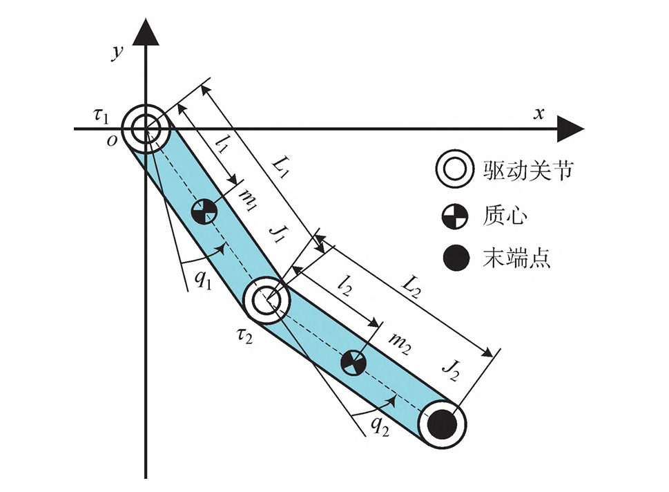
Consider a planar 2-DOF underactuated AI robot in the \(o-xy\) plane, consisting of two links with parameters: \(m_i\) (mass), \(L_i\) (length), \(q_i\) (angle), \(J_i\) (moment of inertia), \(l_i\) (distance from joint to center of mass), and \(\tau_i\) (control torque) . The dynamic equation is given by:\(M(q)\ddot{q} + H(q, \dot{q}) = \tau\) where:\(M(q) = \begin{bmatrix} m_1 + m_2 & -m_2 l_2 \sin q_2 \\ -m_2 l_2 \sin q_2 & m_2 l_2^2 + J_2 \end{bmatrix}, \quad H(q, \dot{q}) = \begin{bmatrix} -m_2 l_2 \dot{q}_2^2 \cos q_2 \\ 0 \end{bmatrix}, \quad \tau = \begin{bmatrix} \tau_1 \\ \tau_2 \end{bmatrix}\)\(M(q)\) is the inertia matrix, \(H(q, \dot{q})\) includes Coriolis and centrifugal forces, and \(\tau\) is the control input vector .
2.2 System Classification
Depending on the passive joint position, the system can be:
- Planar Acrobot: Passive first joint (\(\tau = [0, \tau_2]^T\))
- Planar Pendubot: Passive second joint (\(\tau = [\tau_1, 0]^T\)) .
2.3 Underactuated Characteristics
The underactuated constraint equation derived from the dynamic model is:\(M_{uu}\ddot{q}_u + M_{ua}\ddot{q}_a + H_u = 0\) where subscripts u and a denote underactuated and actuated links, respectively. This equation reveals the coupling between link dynamics, which is critical for designing the unified control strategy .
The state of the underactuated link is determined by:\(\begin{cases} \dot{q}_u(t_s) = -\int_0^T \frac{M_{uu}\ddot{q}_a + H_u}{M_{uu}} dt + \dot{q}_{u0} \\ q_u(t_s) = \int_0^T \dot{q}_u dt + q_{u0} \end{cases}\) This highlights the dependency of the underactuated link’s motion on the actuated link’s trajectory .
3. Trajectory Planning and Parameter Optimization
3.1 Two-Stage Trajectory Design
Stage 1: Rapid Actuated Link Control The first-stage trajectory for the actuated link is designed to quickly reach the target position:\(T_{a1}(t) = \begin{cases} q_{a0} + \tilde{q}_r \left( \frac{t}{t_f} – \frac{1}{2\pi} \sin \alpha \right), & 0 \leq t \leq t_f \\ q_{ad}, & t > t_f \end{cases}\) where \(\tilde{q}_r = q_{ad} – q_{a0}\), \(\alpha = 2\pi t / t_f\), and \(t_f\) is the final time. The first and second derivatives ensure continuity:\(\dot{T}_{a1}(t) = \begin{cases} \frac{\tilde{q}_r}{t_f}(1 – \cos \alpha), & 0 \leq t \leq t_f \\ 0, & t > t_f \end{cases}\)\(\ddot{T}_{a1}(t) = \begin{cases} \frac{\tilde{q}_r}{t_f^2}(2\pi \sin \alpha), & 0 \leq t \leq t_f \\ 0, & t > t_f \end{cases}\)
Stage 2: Underactuated Link Stabilization The second-stage trajectory introduces adjustable parameters to control the underactuated link:\(T_{a2}(t) = A_{11} \text{sech}(\alpha_1) + A_{12} \text{sech}(\alpha_2)\) where:\(\alpha_1 = \frac{\lambda(2t – t_{m1})}{t_{m1}}, \quad \alpha_2 = \frac{\lambda(2t – t_f – t_{m1})}{t_f – t_{m1}}\)\(A_{11}\), \(A_{12}\) (amplitudes), \(t_{m1}\) (connection time), and \(\lambda\) (shape parameter) are optimized to stabilize the underactuated link .
Superimposed Trajectory Combining both stages:\(T_a = T_{a1} + T_{a2}\) This trajectory ensures continuous motion and simultaneous control of both links .
3.2 Parameter Optimization via Differential Evolution
The objective is to minimize the evaluation function:\(h = |q_u(t_f) – q_{ud}| + |\dot{q}_u(t_f)|\) using a differential evolution algorithm. The steps include:
- Random initialization of parameters \(\{A_{11}, A_{12}, t_{m1}, t_f\}\).
- Evaluation of h using the dynamic model.
- Iterative mutation, crossover, and selection to minimize h .
4. Trajectory Tracking Control
4.1 Sliding-Mode Controller Design
Define the state vector \(x = [q_1, q_2, \dot{q}_1, \dot{q}_2]^T\). The state-space equation is:\(\dot{x} = f_a(x) + g_a(x)\tau_a\) where:\(f_a(x) = -M^{-1}(q)H(q, \dot{q}), \quad g_a(x) = -M^{-1}(q)\)
The sliding surface is:\(S_a = \mu_a e_a(t) + \dot{e}_a(t), \quad e_a(t) = T_{ad} – T_a(t)\) with \(\mu_a > 0\) as a design parameter. Differentiating \(S_a\):\(\dot{S}_a = \mu_a \dot{e}_a + \ddot{e}_a = \mu_a \dot{e}_a + f_a(x) + g_a(x)\tau_a – \ddot{T}_a(t)\)
Setting the reaching law as:\(\dot{S}_a = -\zeta_a S_a – \xi_a \text{sgn}(S_a)\) yields the control torque:\(\tau_a = \frac{-\zeta_a S_a – \xi_a \text{sgn}(S_a) – \mu_a \dot{e}_a – f_a(x) + \ddot{T}_a(t)}{g_a(x)}\) where \(\zeta_a, \xi_a > 0\) ensure convergence .
4.2 Stability Analysis
Using the Lyapunov function \(V = \frac{1}{2}S_a^2\), its derivative is:\(\dot{V} = S_a \dot{S}_a = -\zeta_a S_a^2 – \xi_a |S_a| \leq 0\) By LaSalle’s invariance principle, \(S_a \to 0\), implying \(e_a(t) \to 0\) exponentially:\(e_a(t) = e_a(0)e^{-\mu_a t}\) This confirms asymptotic stability of the tracking error .
5. Simulation Experiments
5.1 Setup and Parameters
Simulations are conducted using MATLAB/Simulink for both Acrobot and Pendubot structures with parameters:\(m_i = 1.0 \, \text{kg}, \, L_i = 1.0 \, \text{m}, \, l_i = 0.5 \, \text{m}, \, J_i = 0.083 \, \text{kg·m}^2\) Controller parameters: \(\mu_a = 2.0\), \(\zeta_a = 1.8\), \(\xi_a = 1.2\). Optimization parameters: population size \(N = 40\), mutation rate \(p_m = 0.3\), crossover rate \(p_c = 0.7\), maximum iterations \(G_{\text{max}} = 200\) .
5.2 Results and Comparison
Planar Acrobot
- Initial angles: \(q_1 = q_2 = 0\), Target angles: \(q_1 = -2.0 \, \text{rad}\), \(q_2 = 14.1 \, \text{rad}\)
- Optimized parameters: \(A_{11} = 0.379\), \(A_{12} = -0.936\), \(t_{m1} = 2.245 \, \text{s}\), \(t_f = 7.669 \, \text{s}\)
- Results: Both links reach targets with angular velocities < ±5 rad/s and torque < ±4 N·m, outperforming [8] in control time and stability .
Planar Pendubot
- Initial angles: \(q_1 = q_2 = 0\), Target angles: \(q_1 = 0.5 \, \text{rad}\), \(q_2 = -1.0 \, \text{rad}\)
- Optimized parameters: \(A_{11} = -0.194\), \(A_{12} = -0.066\), \(t_{m1} = 5.808 \, \text{s}\), \(t_f = 11.862 \, \text{s}\)
- Results: Angular velocities < ±1 rad/s, torque < ±1.5 N·m, superior to [14] in smoothness and torque magnitude .
Performance Comparison
| Strategy | Structure | Control Time (s) | Max Torque (N·m) | Max Angular Velocity (rad/s) |
|---|---|---|---|---|
| Proposed | Acrobot | 7.669 | ±4 | ±5 |
| [8] | Acrobot | 10.0+ | ±6 | ±8 |
| Proposed | Pendubot | 11.862 | ±1.5 | ±1 |
| [14] | Pendubot | 15.0+ | ±2.0 | ±2 |
6. Conclusion
This paper presents a unified control strategy for planar 2-DOF underactuated AI robots, combining trajectory planning, parameter optimization, and sliding-mode control. The strategy effectively handles both Acrobot and Pendubot structures by leveraging their coupling dynamics, achieving stable control with reduced torque and shorter settling times. Simulation results validate its superiority over existing methods, paving the way for more robust control of underactuated AI robots in complex environments. Future work will extend this approach to multi-DOF underactuated systems and real-world AI robot applications.