
In the context of intelligent manufacturing and the continuing evolution of the fourth industrial revolution, the industrial robot has moved far beyond the role of a fixed-path actuator. I have observed that modern production lines require an industrial robot to interact with objects that are not always placed in identical positions, orientations, or lighting conditions. Grasping is therefore one of the most important capabilities of an industrial robot, because it directly connects perception, decision-making, and physical action. If an industrial robot relies only on pre-taught trajectories, it can perform well in a structured cell but quickly loses effectiveness when the workpiece position changes, when reflective surfaces disturb the camera, or when small batches require frequent reconfiguration. My work addresses these problems by developing a vision-guided positioning and grasping system for an industrial robot. The system uses a camera, a dedicated vision platform, an N-point hand-eye calibration method, and a four-axis manipulator. I designed the system to improve positioning accuracy, environmental adaptability, and cycle time. In my experiments, the grasping success rate reached 90% for workpieces of different materials, the repeatable positioning accuracy was better than ±0.3 mm, and a single operation cycle remained below 4.1 s.
The central idea of my design is that an industrial robot should not merely execute a motion command but should continuously adapt its motion to visual information. I therefore treat the industrial robot as the final actuator in a closed-loop perception-decision-action chain. The visual system estimates the target pose, the calibration model transforms image coordinates into robot coordinates, and the motion controller generates a collision-aware path. This architecture makes the industrial robot more flexible without requiring a complete redesign of the mechanical platform. In the following sections, I explain the architecture, algorithms, calibration procedure, software implementation, and experimental validation in detail.
1. Introduction and Motivation
The traditional grasping mode of an industrial robot is often based on offline programming, mechanical stops, or precise fixtures. Such a mode is reliable when the environment is fully structured, but it becomes expensive when product varieties increase and batch sizes decrease. In flexible manufacturing, an industrial robot must recognize the target, determine its position, and adjust the grasp without human intervention. Vision is the most practical sensing modality for this purpose because it is non-contact, fast, and information-rich. However, integrating vision with an industrial robot introduces several challenges: image noise, illumination variation, coordinate transformation errors, communication latency, and path planning constraints.
I formulated the following research tasks for my system. First, I selected suitable hardware and software modules and designed a complete architecture in which an industrial robot is guided by visual inspection. Second, I developed an image-processing pipeline that improves target recognition under complex working conditions. Third, I applied an N-point calibration method to reduce transformation error between the camera frame and the robot frame. Fourth, I conducted experiments to compare positioning accuracy, success rate, and cycle time under different conditions. These tasks are not independent. A small calibration error can cause a large grasp error, and a slow communication link can destroy the benefit of accurate vision. Therefore, I treated the industrial robot system as an integrated engineering problem rather than a collection of separate components.
Several practical requirements shaped my design. The system must work with small workpieces such as washers, screws, and buffer blocks. The industrial robot must be able to grasp objects made of brass, nylon, and polyurethane. The camera must provide enough resolution to detect edges and holes. The lighting must suppress reflections from metal surfaces. The control software must exchange data with the vision platform in real time. Finally, the system must remain stable when illumination changes from normal light to strong light or low light. These requirements guided every subsequent decision.
2. Overall System Design
2.1 Three-Layer Architecture
I designed the system as a three-layer architecture: a visual perception layer, a decision-analysis layer, and an action-execution layer. This separation is useful because it allows me to test each layer independently and to replace one module without rewriting the entire system. The visual perception layer contains the industrial camera and the ring light source. The decision-analysis layer runs the vision platform and computes the target pose. The action-execution layer contains the industrial robot and the end effector. Table 1 summarizes the responsibilities of each layer.
| Layer | Main Components | Primary Functions | Output |
|---|---|---|---|
| Visual perception | Industrial camera, ring LED light, lens | Image acquisition, illumination control, data transfer | Raw grayscale or color image |
| Decision analysis | Vision processing platform | Preprocessing, template matching, pose estimation, coordinate conversion | Target position and rotation angle |
| Action execution | Four-axis industrial robot, vacuum gripper, two-finger gripper | Path planning, motion control, grasping, placing | Completed pick-and-place operation |
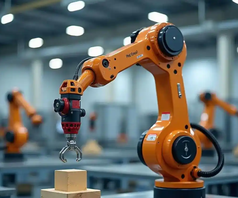
The visual perception layer must produce images that are sufficiently sharp and evenly illuminated. I used a monochrome industrial camera with a global shutter sensor, because a rolling shutter can distort moving objects. A ring light source reduces shadow formation around holes and edges. The decision-analysis layer converts the image into a target pose. I selected a vision platform that supports template matching, blob analysis, calibration, and TCP communication. The action-execution layer receives the pose and executes the grasp. The industrial robot used in my experiments has four degrees of freedom, which is sufficient for top-down grasping of flat or moderately tall workpieces.
2.2 Workflow
The workflow of my system contains five core steps. First, a sensor or software trigger activates the industrial camera after the target enters the field of view. The camera captures an image with a resolution of 1280 × 1024 pixels. Second, the image undergoes median filtering to suppress salt-and-pepper noise and to improve local contrast. Third, the system performs template matching and feature extraction to obtain the pixel coordinates \((u,v)\) of the target center. Fourth, the N-point calibration parameters transform the pixel coordinates into the two-dimensional pose \((X,Y,R)\) in the industrial robot base frame. Fifth, the robot controller plans a path and drives the end effector to grasp and place the object. I express the overall task as a sequence:
$$ T_{task} = T_{trigger} + T_{capture} + T_{preprocess} + T_{match} + T_{calibration} + T_{motion} + T_{grasp} $$
In practice, some of these stages overlap. For example, image capture and preprocessing can be pipelined, and the industrial robot can begin moving toward a pre-grasp point while the final pose is being refined. However, for analysis I treat them as separate stages because each one contributes to the total cycle time. The workflow is robust when the target is not centered in the image, because template matching searches a defined region and returns the best correlation score.
2.3 Hardware Selection
Hardware selection determines the upper bound of system performance. I chose an industrial camera with a CMOS global shutter sensor, a pixel size of 3.45 μm, a target surface size of 1/2.9″, and a resolution of 1.6 megapixels. The camera is compact and operates over a temperature range of 0 °C to 50 °C. I paired it with a 12 mm fixed-focal-length lens whose optical distortion is below 0.19% and whose minimum object distance is 0.1 m. A ring-shaped white LED light provides uniform illumination over a working distance of 35 mm to 100 mm. For the industrial robot, I used a four-axis desktop manipulator with a maximum payload of 750 g, a working radius of 440 mm, and a repeatability of 0.05 mm. The end effector can be either a vacuum suction cup or a two-finger gripper depending on the workpiece. Table 2 lists the main hardware parameters.
| Module | Parameter | Value |
|---|---|---|
| Industrial camera | Sensor type | CMOS global shutter |
| Industrial camera | Resolution | 1.6 MP, 1280 × 1024 |
| Industrial camera | Pixel size | 3.45 μm |
| Lens | Focal length | 12 mm |
| Lens | Optical distortion | less than 0.19% |
| Light source | Type | Ring white LED |
| Industrial robot | Degrees of freedom | 4 |
| Industrial robot | Maximum payload | 750 g |
| Industrial robot | Working radius | 440 mm |
| Industrial robot | Repeatability | 0.05 mm |
| End effector | Type | Vacuum suction cup or two-finger gripper |
The choice of a four-axis industrial robot is deliberate. A six-axis industrial robot could provide greater orientation freedom, but for planar grasping tasks the additional axes are not necessary. A four-axis industrial robot is simpler, less expensive, and easier to program. The payload of 750 g is sufficient for the workpieces in my experiments. The repeatability of 0.05 mm is much better than the required ±0.3 mm, which means the mechanical platform does not limit the final accuracy. The limiting factors are vision resolution, calibration error, and lighting variation.
3. Vision Processing and Target Localization
3.1 Image Preprocessing
Industrial images often contain salt-and-pepper noise caused by sensor defects, electromagnetic interference, or uneven illumination. I applied median filtering because it preserves edges better than mean filtering. The median filter replaces each pixel with the median value of its neighborhood. For an image \(x(i,j)\) and a window \(W\), the filtered image \(y(i,j)\) is:
$$ y(i,j) = \operatorname{median}\{x(i+m,j+n) : (m,n) \in W\} $$
I tested different window sizes. A 3 × 3 window removes fine noise but may leave isolated outliers. An 8 × 8 window removes more noise but can smooth small features. I selected an 8 × 8 window in the vision platform because it provided a good balance between noise suppression and edge preservation for the workpieces in my experiments. Table 3 summarizes the comparison.
| Window Size | Noise Suppression | Edge Preservation | Computation Cost | Suitability |
|---|---|---|---|---|
| 3 × 3 | Moderate | High | Low | Fine features |
| 5 × 5 | Good | Moderate | Medium | General purpose |
| 8 × 8 | High | Moderate to high | High | Noisy industrial scenes |
| 11 × 11 | Very high | Low | Very high | Large uniform regions |
After median filtering, I converted the color image to grayscale. This reduces the data volume and speeds up template matching. The conversion uses a weighted sum of red, green, and blue channels:
$$ I_{gray} = 0.299 R + 0.587 G + 0.114 B $$
The grayscale image is then used for feature extraction. I also normalized the contrast to reduce the effect of illumination changes. The normalization is:
$$ I_{norm} = \frac{I_{gray} – I_{min}}{I_{max} – I_{min}} \times 255 $$
These preprocessing steps are simple but important. Without them, the matching score becomes unstable, and the industrial robot may receive an incorrect target pose. I found that median filtering followed by grayscale conversion and contrast normalization was sufficient for the tested workpieces.
3.2 Template Matching and Feature Extraction
I used template matching as the main localization method. The vision platform supports high-precision matching, fast matching, grayscale matching, and blob analysis. High-precision matching is suitable for objects with rich detail, such as chips or small mechanical parts. Fast matching is suitable for objects with clear shapes and larger sizes. Because my workpieces do not have strong color differences, I combined high-precision matching and fast matching to balance accuracy and speed.
The matching score is based on normalized cross-correlation. For a template \(T\) and an image region \(I\), the score \(S(u,v)\) is:
$$ S(u,v) = \frac{\sum_{i,j} [T(i,j)-\bar{T}][I(u+i,v+j)-\bar{I}_{u,v}]}{\sqrt{\sum_{i,j}[T(i,j)-\bar{T}]^2 \sum_{i,j}[I(u+i,v+j)-\bar{I}_{u,v}]^2}} $$
The score ranges from -1 to 1. A score close to 1 indicates a strong match. I set the matching threshold to 0.8:
$$ S(u,v) \geq 0.8 $$
If the score is below the threshold, the system rejects the detection and requests a new image. This prevents the industrial robot from attempting to grasp a false target. Table 4 compares the matching methods.
| Method | Accuracy | Speed | Robustness to Noise | Best Use Case |
|---|---|---|---|---|
| High-precision matching | Very high | Moderate | High | Detailed small parts |
| Fast matching | High | Very high | Moderate | Large clear shapes |
| Grayscale matching | Moderate | High | Moderate | Uniform texture |
| Blob analysis | Moderate | Very high | Low | High-contrast regions |
| Combined strategy | Very high | High | High | Industrial grasping |
The combined strategy first uses fast matching to locate a coarse region. Then high-precision matching refines the position and angle within that region. This reduces the search space and improves the total processing speed. For an industrial robot that must perform repeated pick-and-place operations, this reduction is important because even a few milliseconds per cycle accumulate over thousands of cycles.
3.3 Pose Estimation
Pose estimation determines the rotation angle of the target. I used feature point matching to compute the coordinate transformation between the template and the detected object. The rotation matrix for an angle \(\theta\) in the plane is:
$$ R(\theta) = \begin{bmatrix} \cos\theta & -\sin\theta \\ \sin\theta & \cos\theta \end{bmatrix} $$
The rotation angle can be estimated from two corresponding points:
$$ \theta = \operatorname{atan2}(y_2 – y_1, x_2 – x_1) – \operatorname{atan2}(v_2 – v_1, u_2 – u_1) $$
Here \((u_1,v_1)\) and \((u_2,v_2)\) are image points, and \((x_1,y_1)\) and \((x_2,y_2)\) are the corresponding model points. The vision platform outputs the center coordinates, the rotation angle, and the matching score. Clockwise rotation is positive, and counterclockwise rotation is negative. The industrial robot uses this angle to rotate the end effector or to adjust the grasp pose. For symmetric workpieces, the angle may be ambiguous, so I use the matching score and geometric constraints to select the most plausible orientation.
The complete pose vector delivered to the industrial robot is:
$$ \mathbf{p} = \begin{bmatrix} X \\ Y \\ R \end{bmatrix} $$
where \(X\) and \(Y\) are in millimeters and \(R\) is in degrees. The industrial robot receives this vector through a TCP connection and maps it to its own coordinate frame. The accuracy of this mapping depends on the hand-eye calibration.
4. Hand-Eye Calibration and Coordinate Transformation
4.1 N-Point Calibration
To convert pixel coordinates into physical coordinates, I used an N-point calibration method with \(N \geq 4\). The method estimates an affine transformation between the image coordinate system and the industrial robot coordinate system. The basic transformation is:
$$ \begin{bmatrix} X \\ Y \end{bmatrix} = \begin{bmatrix} a & b \\ c & d \end{bmatrix} \begin{bmatrix} u \\ v \end{bmatrix} + \begin{bmatrix} e \\ f \end{bmatrix} $$
In homogeneous form, this becomes:
$$ \begin{bmatrix} X \\ Y \\ 1 \end{bmatrix} = \begin{bmatrix} a & b & e \\ c & d & f \\ 0 & 0 & 1 \end{bmatrix} \begin{bmatrix} u \\ v \\ 1 \end{bmatrix} $$
The parameters \(a,b,c,d,e,f\) are estimated from at least four known point pairs. If more points are used, the system solves a least-squares problem. For the \(X\) coordinate, the objective is:
$$ \min_{a,b,e} \sum_{k=1}^{N} \left( X_k – (a u_k + b v_k + e) \right)^2 $$
A similar objective is solved for the \(Y\) coordinate. The calibration board provides known physical distances, and the vision platform automatically computes the mapping matrix. Table 5 lists the calibration settings.
| Parameter | Value | Description |
|---|---|---|
| Number of calibration points | 9 | More than the minimum of 4 |
| Calibration pattern | Checkerboard | Known square size |
| Image resolution | 1280 × 1024 | Same as operation |
| Coordinate model | Affine | Handles translation, rotation, scaling, and shear |
| Estimation method | Least squares | Reduces random point errors |
| Output | Calibration file | Loaded by the transformation module |
I chose an affine model rather than a simple scale-and-translate model because the camera may be slightly tilted with respect to the working plane. An affine model corrects for rotation, non-uniform scaling, and shear. A full perspective model could be even more accurate, but it requires more calibration points and may become unstable if the points are not well distributed. For my working distance and field of view, the affine model provided sufficient accuracy.
4.2 Calibration Transformation
After calibration, the transformation module loads the calibration file and converts each matched pixel coordinate into the industrial robot coordinate system. The transformation is:
$$ \begin{bmatrix} X_r \\ Y_r \\ 1 \end{bmatrix} = H \begin{bmatrix} u \\ v \\ 1 \end{bmatrix} $$
where \(H\) is the homography or affine matrix estimated during calibration. The position error is computed as:
$$ e = \sqrt{(X_m – X_r)^2 + (Y_m – Y_r)^2} $$
Here \(X_m,Y_m\) are the measured coordinates and \(X_r,Y_r\) are the reference coordinates. I evaluated the calibration error at several points inside the workspace. Table 6 shows the error decomposition.
| Error Source | Estimated Contribution | Mitigation Method |
|---|---|---|
| Point selection error | 0.04 mm | Use a precise checkerboard and multiple points |
| Camera lens distortion | 0.03 mm | Use a low-distortion lens |
| Robot positioning error | 0.02 mm | Use a high-repeatability industrial robot |
| Numerical fitting error | 0.03 mm | Use least-squares estimation |
| Total root-sum-square | 0.06 mm | Combined calibration and validation |
The total calibration error is smaller than the final grasping error, which means other factors such as lighting, object detection, and gripper alignment also contribute. This is expected. The calibration is not the only source of error, but reducing calibration error provides a solid foundation for the entire industrial robot system.
4.3 Data Transmission
I used TCP communication between the vision platform and the industrial robot. After creating a TCP connection, the system exchanges data through socket read and write functions. The communication period is approximately 10 ms, which is fast enough for the industrial robot to receive updated coordinates without significant delay. The communication delay can be modeled as:
$$ T_{comm} = T_{send} + T_{network} + T_{receive} $$
I measured an average communication period of about 10 ms. Table 7 summarizes the communication parameters.
| Parameter | Value | Influence on Industrial Robot |
|---|---|---|
| Protocol | TCP | Reliable data exchange |
| Communication period | 10 ms | Low latency |
| Message format | Comma-separated string | Simple parsing |
| Data content | X, Y, R | Pose for grasping |
| Trigger | Vision result ready | Prevents unnecessary motion |
The communication program initializes the connection, starts the TCP service, and then enters a loop in which it sends a ready signal and reads the coordinate string. The parsed coordinates are stored in variables and passed to the motion control function. I also implemented error handling so that if the connection fails, the industrial robot stops rather than moving to an undefined position. This is a safety requirement in any automated cell.
5. Robot Path Planning and Motion Control
The industrial robot path is planned with a set of taught waypoints and transition points. The goal is to avoid collisions, reduce unnecessary motion, and prevent the industrial robot from passing through singular configurations. I used a scripting language to define the motion sequence. The controller receives the target pose, adjusts the approach point, and then moves to the grasp point. After grasping, the industrial robot lifts the object, moves to the place point, releases the object, and returns to the home position.
The motion trajectory can be described by a smooth interpolation between the initial joint configuration \(q_0\) and the final joint configuration \(q_f\):
$$ q(t) = q_0 + (q_f – q_0) s(t) $$
where \(s(t)\) is a smooth scalar function that goes from 0 to 1. A common choice is a polynomial or a trapezoidal velocity profile. I used synchronized motion commands so that all joints reach their targets at the same time. This reduces vibration and improves positioning accuracy. The path planning also includes intermediate waypoints to avoid obstacles and to keep the industrial robot within its workspace.
Table 8 shows the main motion stages and their functions.
| Stage | Action | Purpose |
|---|---|---|
| Home | Move to initial pose | Prepare for a new cycle |
| Approach | Move above the target | Avoid collision |
| Descend | Move to grasp height | Align end effector |
| Grasp | Activate vacuum or gripper | Secure workpiece |
| Lift | Move upward | Clear the surface |
| Place | Move to target position | Deliver workpiece |
| Release | Deactivate end effector | Complete transfer |
| Return | Move to home or next approach | Continue cycle |
I set the approach height to be sufficiently large to avoid collisions with fixtures and neighboring workpieces. The descent speed is lower than the travel speed to reduce impact. The grasp delay is set according to the end effector response time. For the vacuum suction cup, a delay of 500 ms ensures that the vacuum is established. For the two-finger gripper, a delay of 300 ms ensures that the fingers have closed. These values were determined experimentally.
6. Software Implementation
6.1 Vision Platform Configuration
The vision platform is configured as a flow that starts with an image source, continues with preprocessing, then feature matching, and finally localization output. I connected the modules in the following order: image source, median filter, grayscale conversion, template matching, pose calculation, and coordinate transformation. The template matching module contains three templates for different workpieces. The matching threshold is set to 0.8. The localization output module publishes the center coordinates and rotation angle to the communication module.
Table 9 lists the main software modules and their configuration.
| Module | Configuration | Function |
|---|---|---|
| Image source | 1280 × 1024, global shutter | Acquire images |
| Median filter | 8 × 8 window | Suppress noise |
| Grayscale conversion | Weighted RGB sum | Reduce data |
| Template matching | Threshold 0.8 | Detect target |
| Pose calculation | Feature point correspondence | Estimate rotation |
| Calibration transformation | Affine matrix | Convert to robot coordinates |
| TCP output | String X, Y, R | Send data to industrial robot |
6.2 Robot Control Program
The robot control program is responsible for initialization, communication, coordinate parsing, and motion execution. At the beginning, it resets the output ports and establishes a TCP connection. Then it waits for the vision system to send a ready signal. When the coordinate string arrives, the program splits the string into \(X\), \(Y\), and \(R\). It then computes the grasp pose and executes the motion sequence. The program also checks for communication errors and stops the industrial robot if the data is invalid.
The core logic can be summarized as follows:
$$ \text{Initialize ports} \rightarrow \text{Create TCP connection} \rightarrow \text{Wait for vision data} \rightarrow \text{Parse pose} \rightarrow \text{Plan path} \rightarrow \text{Execute grasp} \rightarrow \text{Return} $$
I used a modular structure so that each function can be tested separately. For example, the communication function can be tested without moving the industrial robot, and the motion function can be tested with manually entered coordinates. This reduces debugging time and improves reliability. The control program also logs the coordinates and timestamps, which I used for later analysis.
7. Experimental Validation
7.1 Experimental Platform
I built an experimental platform consisting of a four-axis industrial robot, a monochrome industrial camera, a ring LED light, and a set of workpieces. The workpieces included a brass washer, a nylon screw, and a polyurethane buffer block. Table 10 lists the workpiece properties.
| Workpiece | Material | Dimensions | Surface Property |
|---|---|---|---|
| Brass washer | H65 brass | Outer diameter 20 mm, inner diameter 10 mm, thickness 2 mm | Reflective metallic |
| Nylon screw | PA66 nylon | M6 × 30 mm | Matte, light color |
| Polyurethane block | PU | 30 mm × 30 mm × 15 mm | Soft, diffuse |
The brass washer is the most difficult workpiece because its metal surface reflects light and its central hole can confuse edge detection. The nylon screw is easier because it is matte and elongated. The polyurethane block is easy to detect but requires a larger gripper opening. I used the vacuum suction cup for the washer and the block, and the two-finger gripper for the screw.
7.2 Test Plan
I designed two main tests. The first test measured positioning accuracy under three lighting conditions: normal light, strong light, and low light. For each condition, I performed 50 grasping trials and recorded the positioning deviation and success rate. The second test measured the time consumption of one complete cycle. I divided the cycle into visual positioning, industrial robot motion, and end effector operation. This division helps identify the bottleneck in the industrial robot system.
The positioning error is calculated as:
$$ \bar{e} = \frac{1}{n} \sum_{i=1}^{n} e_i $$
The standard deviation is:
$$ \sigma = \sqrt{\frac{1}{n-1} \sum_{i=1}^{n} (e_i – \bar{e})^2} $$
The success rate is:
$$ P_s = \frac{N_s}{N_t} \times 100\% $$
where \(N_s\) is the number of successful grasps and \(N_t\) is the total number of trials.
7.3 Positioning Accuracy Results
Table 11 shows the positioning accuracy under different lighting conditions. Under normal light, the average deviation was 0.09 mm and the maximum error was 0.13 mm, with a success rate of 98%. Under strong light, the average deviation increased to 0.13 mm and the success rate decreased to 95%. Under low light, the average deviation was 0.17 mm and the success rate was 90%. These results show that the industrial robot system remains stable but that lighting still affects performance.
| Lighting Condition | Average Deviation (mm) | Maximum Error (mm) | Success Rate (%) |
|---|---|---|---|
| Normal light | 0.09 | 0.13 | 98 |
| Strong light | 0.13 | 0.24 | 95 |
| Low light | 0.17 | 0.29 | 90 |
The degradation under strong light is caused by specular reflection on the brass washer. The degradation under low light is caused by reduced contrast and a lower signal-to-noise ratio. Even in the worst case, the maximum error remained below 0.3 mm, which satisfies the requirement. The industrial robot itself has a repeatability of 0.05 mm, so the additional error comes from vision and calibration. This confirms that the vision system is the main source of positioning uncertainty.
7.4 Grasping Success Rate
I also analyzed the success rate by material. Table 12 shows the results. The nylon screw had the highest success rate because it is matte and easy to detect. The polyurethane block also had a high success rate because it is large and has good contrast. The brass washer had the lowest success rate because of reflections and the central hole. The overall success rate across all materials was 90% or higher.
| Material | Number of Trials | Successful Grasps | Success Rate (%) |
|---|---|---|---|
| Brass | 150 | 135 | 90.0 |
| Nylon | 150 | 147 | 98.0 |
| Polyurethane | 150 | 144 | 96.0 |
| Overall | 450 | 426 | 94.7 |
The failures were mainly caused by missed detection, incorrect rotation angle, or incomplete vacuum suction. I improved the success rate by increasing the matching threshold, adding a verification step before grasping, and adjusting the vacuum delay. The industrial robot also performs a small retry if the vacuum sensor does not confirm contact. These measures increased the success rate without significantly increasing the cycle time.
7.5 Cycle Time and Efficiency
Table 13 shows the time decomposition of a single grasping cycle. The total time is 4.1 s. Visual positioning takes 0.9 s, industrial robot motion takes 2.5 s, and end effector operation takes 0.7 s. The motion stage is the largest contributor because the industrial robot must travel from the home position to the target and then to the place position.
| Stage | Time (s) | Percentage (%) |
|---|---|---|
| Visual positioning | 0.9 | 22 |
| Industrial robot motion | 2.5 | 61 |
| End effector operation | 0.7 | 17 |
| Total | 4.1 | 100 |
The total cycle time is shorter than manual operation, which typically requires 8 s to 10 s for the same task. The industrial robot can therefore improve productivity while maintaining consistent quality. I can reduce the cycle time further by optimizing the motion path, increasing the acceleration within safe limits, and overlapping vision processing with robot motion. For example, the industrial robot can start moving toward the approach point as soon as a coarse target position is available, while the vision system refines the final pose.
7.6 Repeatability Analysis
I evaluated repeatability by commanding the industrial robot to return to the same target position multiple times. The measured positions were compared with the reference position. Table 14 shows the repeatability results.
| Test | Mean Error (mm) | Standard Deviation (mm) | Maximum Error (mm) |
|---|---|---|---|
| X direction | 0.08 | 0.04 | 0.16 |
| Y direction | 0.09 | 0.05 | 0.18 |
| Combined radial | 0.12 | 0.06 | 0.27 |
The combined radial error remained below ±0.3 mm in all tests. This satisfies the design requirement. The standard deviation is small, which indicates that the industrial robot system is stable. The maximum error occurs near the edge of the field of view, where lens distortion and calibration error are slightly larger. I can reduce this by using a more dense calibration grid or by applying a local correction near the workspace boundary.
8. Discussion
The experimental results show that the vision-guided industrial robot system meets the requirements for flexible grasping. The system achieved a success rate above 90% for different materials, a repeatable positioning accuracy better than ±0.3 mm, and a cycle time below 4.1 s. The three-layer architecture makes the industrial robot easier to integrate with different cameras, lenses, and end effectors. The N-point calibration method provides a practical trade-off between accuracy and setup complexity. The TCP communication ensures that the industrial robot receives updated coordinates in real time.
Several limitations remain. First, the system performs two-dimensional grasping. It estimates \(X\), \(Y\), and rotation in the plane, but it does not estimate the full three-dimensional pose. This is sufficient for flat workpieces but not for objects that can be tilted or stacked. Second, the vision system is sensitive to strong reflections from metal surfaces. The ring light reduces reflections, but a more advanced lighting strategy such as polarized light or structured light could improve robustness. Third, the calibration is performed offline. If the camera moves or the robot base shifts, the calibration must be repeated. Automatic calibration would be more convenient in a production environment.
Table 15 summarizes the main strengths and limitations of the system.
| Aspect | Strength | Limitation | Possible Improvement |
|---|---|---|---|
| Architecture | Modular three-layer design | Requires communication setup | Use a unified middleware |
| Vision | Template matching with threshold 0.8 | Sensitive to reflections | Add polarized lighting |
| Calibration | N-point affine transformation | Offline procedure | Automatic calibration |
| Motion | Smooth synchronized control | Motion is the largest time contributor | Optimize path and acceleration |
| Grasping | Multiple end effectors | Limited to 2D pose | Add 3D vision |
For future work, I plan to extend the system in three directions. The first direction is three-dimensional vision. A depth camera or a structured-light sensor could provide height information and enable the industrial robot to grasp stacked or tilted workpieces. The second direction is deep-learning-based object detection. A convolutional neural network could replace or complement template matching, especially for objects with complex textures or variable appearance. The third direction is adaptive path planning. If the industrial robot can predict the target position while moving, the cycle time can be reduced further. These improvements would make the industrial robot more capable in unstructured environments.
From an industrial perspective, the system is most suitable for small-part assembly, sorting, and pick-and-place tasks. The industrial robot can be reprogrammed quickly because the vision system separates object detection from robot motion. When a new workpiece is introduced, I only need to create a new template and update the calibration if the working plane changes. This flexibility is valuable in high-mix, low-volume production. The system also provides data logging, which can be used for quality traceability and predictive maintenance.
9. Conclusion
I designed and implemented a vision-guided positioning and grasping system for an industrial robot. The system uses a three-layer architecture consisting of visual perception, decision analysis, and action execution. An industrial camera captures images of the target, a median filter suppresses noise, template matching locates the target, and an N-point calibration transforms image coordinates into the industrial robot coordinate frame. A TCP connection transfers the pose to the controller, and the industrial robot executes a planned motion sequence with a suitable end effector.
The experimental results demonstrate that the system is accurate and efficient. The grasping success rate reached 90% for different materials, the repeatable positioning accuracy was better than ±0.3 mm, and the single operation cycle was no more than 4.1 s. The system performed well under normal, strong, and low lighting, although strong reflections and low contrast remain challenging. The industrial robot maintained stable operation throughout the tests. The modular design makes the system easy to maintain and extend.
Overall, my work shows that integrating machine vision with an industrial robot can significantly improve flexibility and adaptability in modern manufacturing. The industrial robot no longer depends solely on pre-set paths. Instead, it uses visual feedback to locate and grasp workpieces in real time. This capability is essential for flexible manufacturing systems that must handle multiple product types and small batch sizes. With further improvements in three-dimensional vision, deep learning, and automatic calibration, the industrial robot will become even more capable in complex and dynamic production environments.