
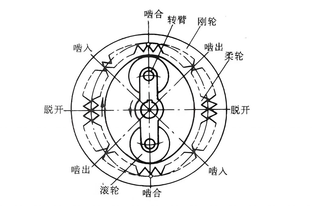
The pursuit of high-performance motion control has consistently driven advancements in precision gearing technology. Among these, the harmonic drive gear stands out for its exceptional capabilities, offering high reduction ratios, compact design, superior positional accuracy, and minimal backlash within a single stage. Its operation hinges on the controlled elastic deformation of a flexible spline, or flexspline, by a wave generator, which creates a moving, elliptical wave that meshes with the teeth of a rigid circular spline. The fidelity of this meshing action, critical for the transmission’s performance and longevity, is fundamentally governed by the precise geometry of the conjugate tooth profiles. Therefore, developing an accurate and practical method to solve for these profiles is paramount in the design of high-quality harmonic drive systems.
My investigation focuses on a robust methodology for determining the conjugate tooth profile of the circular spline based on a known flexspline profile. Traditional theoretical approaches rely on an analytical deformation function for the flexspline derived from elastic shell theory under several simplifying assumptions, such as an inextensible middle surface and straight generators. This function, often involving complex elliptical integrals, is then substituted into the meshing equations derived from envelope theory. While mathematically sound, this method can introduce discrepancies because the assumed theoretical deformation may not perfectly match the actual, more complex deformation state of the flexspline under the influence of the wave generator, especially when considering the presence of teeth. To address this, I propose and implement a comprehensive numerical approach that integrates finite element analysis (FEA), advanced curve fitting, and kinematic simulation to derive a more physically accurate conjugate profile.
The core of the conjugate profile problem lies in the mathematical relationship describing the relative motion between the two gears. In a standard speed-reducing configuration with the circular spline fixed, the wave generator as input, and the flexspline as output, the geometric model for solving the conjugate profile is established. A fixed global coordinate system \( C_G (x_G, y_G) \) is attached to the circular spline, with its origin \( O_G \) at the assembly’s center of rotation and its y-axis aligned with the symmetry line of a circular spline tooth space. A moving coordinate system \( C_R (x_R, y_R) \) is attached to the flexspline, its origin \( O_R \) at the intersection of the tooth symmetry line and the flexspline’s deformed neutral curve \( S_R \). The wave generator has its own coordinate system \( C_0 (x_0, y_0) \). According to envelope theory, the family of curves traced by the flexspline tooth profile in the fixed coordinate system \( C_G \), as the wave generator rotates, must envelop the desired circular spline tooth profile.
The mathematical condition for this envelope, leading to the conjugate profile expression for the circular spline, is given by the following system of equations. The coordinate transformation defines the trajectory, and the envelope condition ensures tangency.
$$
\begin{bmatrix}
x_G(t) \\
y_G(t) \\
1
\end{bmatrix} = \mathbf{M}_{RG} \begin{bmatrix}
x_R(t) \\
y_R(t) \\
1
\end{bmatrix} = \begin{bmatrix}
\cos\varphi & \sin\varphi & \rho \sin\gamma \\
-\sin\varphi & \cos\varphi & \rho \cos\gamma \\
0 & 0 & 1
\end{bmatrix} \begin{bmatrix}
x_R(t) \\
y_R(t) \\
1
\end{bmatrix}
$$
$$
\frac{\partial x_G}{\partial \phi} \frac{\partial y_G}{\partial t} – \frac{\partial y_G}{\partial \phi} \frac{\partial x_G}{\partial t} = 0
$$
Where the key kinematic relationships are:
$$
\varphi = \mu + \gamma = \mu + \frac{U}{z_1} \phi + \frac{\upsilon}{r_m}
$$
$$
\mu = \arctan\left(\frac{\rho’}{\rho}\right) \approx \frac{1}{r_m} \frac{d\omega}{d\phi}
$$
In these equations, \( \rho \) is the polar radius of the deformed flexspline neutral curve, \( \varphi \) is the angle between coordinate systems \( C_R \) and \( C_G \), \( \phi \) is the rotation angle of the wave generator, and \( \gamma \) is the rotation of the flexspline. The term \( U/z_1 \) represents the generalized transmission ratio, with \( U \) being the wave number (typically 2) and \( z_1 \) the number of teeth on the flexspline. The variables \( \omega(\phi) \) and \( \upsilon(\phi) \) are the radial and tangential displacement functions of the flexspline’s neutral surface, respectively, and \( \mu \) is the local tooth inclination angle due to deformation. The symbol \( r_m \) denotes the nominal radius of the flexspline’s middle surface before deformation. Clearly, accurate knowledge of the deformation functions \( \omega(\phi) \) and \( \upsilon(\phi) \) is the critical link between the known flexspline profile and the unknown circular spline profile. Directly solving this system analytically for a given \( \omega(\phi) \) and \( \upsilon(\phi) \) can be algebraically intensive. My approach circumvents this complexity by using numerical methods to first obtain accurate deformation functions and then to solve the envelope condition through simulation.
The first and most crucial step in my methodology is to obtain a high-fidelity representation of the flexspline’s initial, unloaded deformation when assembled with the wave generator. I chose to analyze a common configuration: a cup-type flexspline and a circular spline with a two-arc (“double-circular-arc”) tooth profile, driven by an elliptical cam wave generator. The basic parameters for this case study are summarized in the table below.
| Parameter | Symbol | Value |
|---|---|---|
| Module | \( m \) | 0.5 mm |
| Flexspline Tooth Count | \( z_1 \) | 200 |
| Circular Spline Tooth Count | \( z_2 \) | 202 |
| Radial Deformation Coefficient | \( \omega^* \) | 1.0 |
| Theoretical Radial Deformation | \( w_0 \) | \( m \cdot \omega^* = 0.5 \) mm |
To capture the true deformation state, I constructed a detailed 3D finite element model in Abaqus/Standard. The model included the full cup-type flexspline, complete with its tooth ring, rather than a symmetric segment, to account for any potential asymmetrical effects and the influence of the teeth on the overall deformation field. The material for the flexspline was modeled as 35CrMnSiA steel with an elastic modulus of 209 GPa and a Poisson’s ratio of 0.295. The wave generator assembly was simplified as a single, rigid elliptical ring whose outer contour accounted for the thickness of the flexible bearing. This simplification is valid for analyzing initial assembly deformation without rotational friction. The elliptical profile was defined by offsetting the nominal cam ellipse by half the bearing thickness in the radial direction. The interaction between the wave generator’s outer surface and the flexspline’s inner bore was defined as a surface-to-surface contact pair. A displacement-driven simulation was performed, where the upper and lower halves of the rigid wave generator were moved towards and away from the center, respectively, by the nominal radial deformation amount \( w_0 \), to simulate the assembly process.
The results from the FEA provided profound insights. The deformation was not purely elliptical as often assumed in theoretical models. The radial displacement contour plot revealed a maximum radial expansion of approximately 0.553 mm along the major axis, which is about 10.6% larger than the theoretical 0.5 mm. More notably, at the mouth of the cup along the minor axis, significant inward radial displacement (up to -0.557 mm) was observed, indicating a “pinching” or wrapping effect of the cup opening around the wave generator. This phenomenon is a known contributor to wear in flexible bearings. The tangential displacement plot showed maximum values near \(\pm45^\circ\) from the major axis at the cup mouth, reaching about 0.293 mm, compared to a common theoretical maximum of \( w_0/2 = 0.25 \) mm. These discrepancies underscore the necessity of using FEA-derived data over simplified analytical functions for high-precision harmonic drive gear design.
The next step involved extracting precise deformation data to create continuous mathematical functions. I sampled the radial \( \omega(\phi) \) and tangential \( \upsilon(\phi) \) displacements at nodes located on the neutral surface of the middle cross-section of the flexspline’s tooth ring, all around its circumference. This data set, representing one full mechanical revolution, served as the basis for curve fitting. Given the periodic and smooth nature of the deformation, I selected a sum of sine functions as the fitting model, implemented using MATLAB’s Curve Fitting Toolbox. The general form for both deformation functions is:
$$
f(\phi) = \sum_{i=1}^{n} a_i \sin(b_i \phi + c_i)
$$
Where \( a_i, b_i, c_i \) are the fitting coefficients, and \( \phi \) is the angular position. After evaluating fits with varying numbers of terms (up to 9), a three-term sine series was found to provide an excellent balance between accuracy and model simplicity. The quality of the fit was assessed using standard metrics: Sum of Squares Due to Error (SSE), Root Mean Square Error (RMSE), and R-square. The optimal fitting results are presented in the following tables.
| Coefficient Set | Value |
|---|---|
| \( a_1, a_2, a_3 \) | [0.5272, 0.02677, 0.007596] mm |
| \( b_1, b_2, b_3 \) | [1.987, 5.965, 4.033] rad⁻¹ |
| \( c_1, c_2, c_3 \) | [1.611, 1.694, -9.533] rad |
| SSE | 3.233e-3 mm² |
| RMSE | 4.69e-3 mm |
| Coefficient Set | Value |
|---|---|
| \( a_1, a_2, a_3 \) | [0.2956, 0.01807, 0.01897] mm |
| \( b_1, b_2, b_3 \) | [2.013, 0.2032, 4.067] rad⁻¹ |
| \( c_1, c_2, c_3 \) | [3.09, -1.919, -1.909] rad |
| SSE | 4.515e-3 mm² |
| RMSE | 7.044e-3 mm |
The maximum residual error for the radial fit was 0.00107 mm, which is only about 1/517 of the maximum radial deformation, and for the tangential fit, it was 0.00053 mm, about 1/553 of the maximum tangential deformation. These negligible fitting errors confirm the reliability of the obtained functions \( \omega_{FEA}(\phi) \) and \( \upsilon_{FEA}(\phi) \) as accurate representations of the FEA-derived deformation. They effectively replace the traditional theoretical deformation functions in the subsequent conjugate profile analysis.
With accurate deformation functions in hand, I proceeded to solve for the conjugate circular spline profile. Instead of directly tackling the complex partial differential envelope condition from Equation (2), I employed a kinematic simulation approach combined with numerical envelope extraction. Using a computational script, I simulated the complete meshing cycle of a single flexspline tooth. This involved applying the coordinate transformation from Equation (1), using the fitted functions \( \omega_{FEA}(\phi) \) and \( \upsilon_{FEA}(\phi) \) to define the motion parameters \( \rho, \gamma, \mu \) at each small increment of the wave generator angle \( \phi \). For every \( \phi \), the known double-circular-arc profile of the flexspline tooth was plotted in the fixed global coordinate system \( C_G \). The collection of all these curves for a full engagement/disengagement cycle formed the “curve family” or the motion trajectory of the flexspline tooth relative to the fixed circular spline.
The sought-after conjugate profile of the circular spline is the envelope of this curve family. Mathematically, it is the curve that is tangent to every member of the family. I extracted this envelope numerically from the densely sampled trajectory data. The resulting envelope curve represents the theoretical, geometrically perfect tooth profile for the circular spline that would conjugate with the given flexspline profile under the specified deformation conditions. However, a raw mathematical envelope may contain segments that are impractical for manufacturing (e.g., severely undercut or pointed shapes).
Therefore, the final step was to design a manufacturable profile that closely approximates the theoretical envelope in the active working region. Observing that the envelope in the tooth flank region had a shape conducive to a circular arc, I applied a least-squares fitting routine to approximate the critical working section of the envelope with a smooth arc-line-arc composite curve. This is a common and practical design for double-circular-arc harmonic drive teeth. The deviation between the fitted circular spline profile and the theoretical envelope points was meticulously calculated. The maximum error was found to be a mere 0.00869 µm, with an average error of 0.00576 µm. Compared to standard gear accuracy grades, this error is utterly insignificant (e.g., over 1000 times smaller than the form error tolerance for a precision Grade 6 gear), validating the fitted profile as an excellent engineering approximation of the true conjugate shape.
| Aspect | Theoretical Approach | Proposed FEA-Simulation Method |
|---|---|---|
| Deformation Source | Analytical shell theory (elliptical assumption) | 3D Nonlinear Finite Element Analysis |
| Radial Deformation Max | \(\pm 0.500\) mm | \(+0.553\) mm / \(-0.557\) mm |
| Tangential Deformation Max | \(\sim 0.250\) mm | \(\sim 0.293\) mm |
| Deformation Function | Complex elliptical integral form | Simple sum-of-sines fit: \( \sum a_i \sin(b_i\phi+c_i) \) |
| Profile Solution Method | Analytical solution of meshing equations | Kinematic simulation & numerical envelope extraction |
| Resulting Profile | May not account for real deformation effects | Based on physically accurate deformation; manufacturable fit applied. |
| Primary Advantage | Closed-form solution | High accuracy, accounts for complex 3D effects and tooth influence. |
In conclusion, this work successfully demonstrates a viable and refined methodology for solving conjugate tooth profiles in harmonic drive gears. By integrating finite element analysis to capture the true initial deformation of the flexspline, employing robust curve fitting to create simple and accurate deformation functions, and utilizing kinematic simulation with numerical envelope theory, I have developed a process that overcomes the limitations of purely analytical models. The method directly incorporates the influence of the tooth ring and the complex three-dimensional deformation state, aspects often simplified in classical theory. The final output is a precise, manufacturable circular spline tooth profile that is geometrically conjugate to the given flexspline profile under realistic operating conditions. This integrated FEA-simulation approach provides a powerful and practical tool for the design and analysis of high-performance harmonic drive gear systems, potentially leading to improved meshing quality, reduced wear, and enhanced transmission accuracy. Future work will involve constructing physical prototypes based on these profiles and conducting experimental tests to validate their meshing performance and durability under load.