
In the field of precision mechanical transmissions, strain wave gears, also known as harmonic drives, play a critical role due to their high reduction ratios, compact design, and minimal backlash. However, the longevity and efficiency of these systems heavily depend on the lubrication conditions between the meshing teeth. Traditionally, fluid dynamic lubrication theories applied to strain wave gears have assumed perfectly smooth surfaces, neglecting the inevitable surface roughness present in real-world components. This oversight becomes particularly significant under thin-film lubrication regimes, where roughness effects can dominate and lead to mixed or boundary lubrication states. In this article, we explore the lubrication performance of strain wave gear teeth by incorporating surface roughness effects through the average flow model and the average Reynolds equation. We derive numerical solutions for both shear and squeeze films, present minimum oil film thickness curves, and demonstrate that increased surface roughness can enhance hydrodynamic pressure effects, promoting adequate film formation. Our analysis aims to provide a more accurate predictive tool for designers and engineers working with strain wave gears.
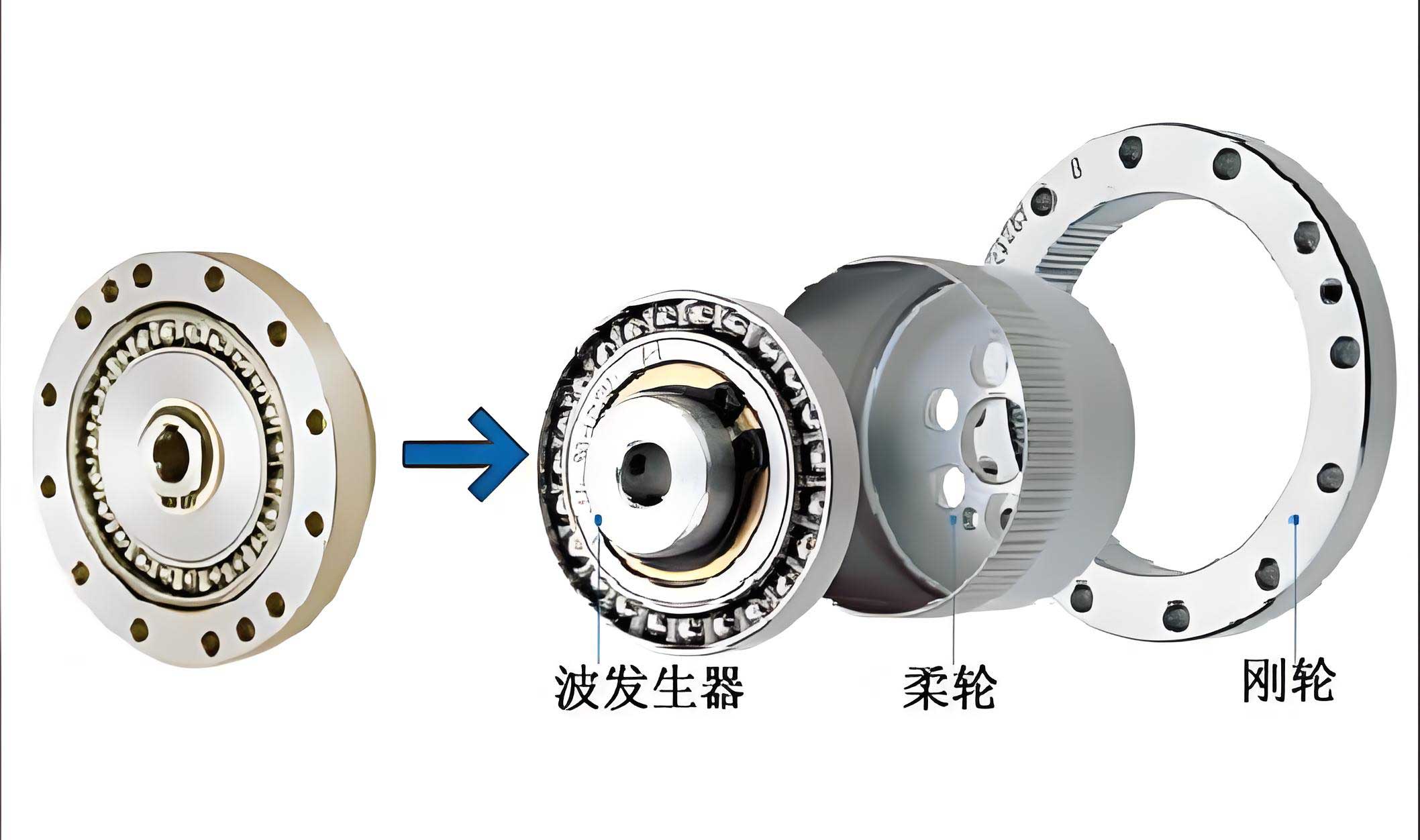
The fundamental lubrication mechanism in strain wave gears arises from the relative motion between the flexible spline (or flexspline) and the circular spline teeth. During operation, the wave generator deforms the flexspline, causing its teeth to engage with those of the circular spline in a progressive manner. This engagement involves both tangential sliding and normal squeezing motions between the tooth surfaces, creating wedge-shaped gaps that are conducive to hydrodynamic lubrication. The resulting oil film is a combination of shear films (due to sliding) and squeeze films (due to approach or separation). To model this, the classical Reynolds equation for smooth surfaces is often used, but it fails to account for roughness when the film thickness is comparable to the surface asperity heights. Therefore, we adopt the average Reynolds equation based on Patir and Cheng’s average flow model, which introduces flow factors to quantify roughness effects.
The two-dimensional, non-isothermal, average Reynolds equation considering surface roughness is given as:
$$ \frac{\partial}{\partial x} \left( \phi_x h^3 \frac{\partial \bar{p}}{\partial x} \right) + \frac{\partial}{\partial y} \left( \phi_y h^3 \frac{\partial \bar{p}}{\partial y} \right) = 6U \eta \frac{\partial \bar{h}_T}{\partial x} + 6U \eta \sigma \frac{\partial \phi_s}{\partial x} + 12 \eta \frac{\partial \bar{h}_T}{\partial t} $$
where \( \bar{p} \) is the average pressure, \( \bar{h}_T \) is the average film thickness accounting for roughness (\( \bar{h}_T = h + \delta_1 + \delta_2 \), with \( h \) as the nominal film thickness, and \( \delta_1, \delta_2 \) as roughness heights), \( \eta \) is the lubricant viscosity, \( U \) is the average surface velocity, \( \phi_x \) and \( \phi_y \) are pressure flow factors, \( \phi_s \) is the shear flow factor, and \( \sigma \) is the composite surface roughness standard deviation. For strain wave gears with similar roughness on both tooth surfaces, the shear flow factor \( \phi_s \) can be neglected, simplifying the equation to:
$$ \frac{\partial}{\partial x} \left( \phi_x h^3 \frac{\partial \bar{p}}{\partial x} \right) + \frac{\partial}{\partial y} \left( \phi_y h^3 \frac{\partial \bar{p}}{\partial y} \right) = 6U \eta \phi_c \frac{\partial h}{\partial x} + 12 \eta \phi_c \frac{\partial h}{\partial t} $$
Here, \( \phi_c \) is the contact factor, which modifies the flow due to roughness interactions. The pressure flow factors \( \phi_x \) and \( \phi_y \) depend on the surface roughness orientation. For isotropic roughness, \( \phi_x = \phi_y = \phi \), and an empirical relation is:
$$ \phi = 1 – 0.9 \exp(-0.56 \lambda) $$
where \( \lambda = h/\sigma \) is the film thickness ratio. The contact factor \( \phi_c \) is calculated as:
$$ \phi_c = \exp[-0.6912 + 0.782 \lambda – 0.304 \lambda^2 + 0.0401 \lambda^3] $$
These factors adjust the lubrication equations to reflect real surface conditions in strain wave gears, moving beyond ideal smooth-surface assumptions.
To solve the average Reynolds equation for strain wave gear teeth, we simplify it by focusing on the specific geometry and motion of the meshing pair. The boundary conditions for the tooth contact region are defined by the engagement depth \( B \) and tooth width \( L \):
$$ x = 0, B; \quad \bar{p} = 0 $$
$$ y = 0, L; \quad \bar{p} = 0 $$
The minimum oil film thickness \( h_{\text{min}} \) is a critical parameter, determined as the combination of shear film and squeeze film contributions, along with effects from the wedge-shaped gap ratio. We express it as:
$$ h_{\text{min}} = h_{q,\text{min}} = h_{y,\text{min}} $$
where \( h_{q,\text{min}} \) is the minimum shear film thickness and \( h_{y,\text{min}} \) is the minimum squeeze film thickness. Since analytical solutions are intractable, we employ numerical methods, starting with dimensionless transformations to generalize the results.
For the shear film component, the average Reynolds equation reduces to:
$$ \frac{\partial}{\partial x} \left( \phi h^3 \frac{\partial \bar{p}}{\partial x} \right) + \frac{\partial}{\partial y} \left( \phi h^3 \frac{\partial \bar{p}}{\partial y} \right) = 6U \eta \phi_c \frac{\partial h}{\partial x} $$
Introducing dimensionless variables: \( x = X \cdot B \), \( y = Y \cdot L \), \( \bar{p} = p \cdot \frac{6U \eta B}{h_1^2} \), \( \beta = \frac{B^2}{L^2} \), and \( h = h_1 \cdot (1 + X) = \bar{h} \cdot h_1 \) (assuming \( h_2 = 2h_1 \)), we derive the dimensionless form:
$$ \frac{\partial^2 p}{\partial X^2} + \beta \frac{\partial^2 p}{\partial Y^2} + \frac{3}{1+X} \frac{\partial p}{\partial X} = \frac{\phi_c}{\phi \bar{h}^3} \frac{d\bar{h}}{dX} $$
Applying the infinite short bearing approximation, where pressure varies parabolically along the \( y \)-direction, we set \( p = p_h (1 – Y^2) \). This reduces the problem to one dimension along \( X \):
$$ \frac{d^2 p_h}{dX^2} + a \frac{d p_h}{dX} + b p_h = c $$
with coefficients:
$$ a = \frac{3}{1+X}, \quad b = -2\beta, \quad c = \frac{\phi_c}{\phi \bar{h}^3} \frac{d\bar{h}}{dX} $$
For the squeeze film component, due to the wedging approach motion, the equation becomes:
$$ \frac{\partial}{\partial x} \left( \phi h^3 \frac{\partial \bar{p}}{\partial x} \right) + \frac{\partial}{\partial y} \left( \phi h^3 \frac{\partial \bar{p}}{\partial y} \right) = 12 \eta \phi_c \frac{\partial h}{\partial t} $$
Dimensionless variables here are: \( x = X \cdot B \), \( y = Y \cdot L \), \( \bar{p} = p \cdot P \), \( \beta = \frac{B^2}{L^2} \), \( h = h_0 \cdot (1 + X) = \bar{h} \cdot h_0 \), and \( t = \frac{12 \eta}{h_0^2} T \), where \( h_0 \) is the initial film thickness and \( T \) is time. The dimensionless form is:
$$ \frac{\partial^2 p}{\partial X^2} + \beta \frac{\partial^2 p}{\partial Y^2} + \frac{3}{1+X} \frac{\partial p}{\partial X} = \frac{\phi_c}{\phi \bar{h}^3} \frac{d\bar{h}}{dT} $$
Similarly, using the parabolic pressure distribution, we obtain:
$$ \frac{d^2 p_h}{dX^2} + a \frac{d p_h}{dX} + b p_h = c $$
with coefficients:
$$ a = \frac{3}{1+X}, \quad b = -2\beta, \quad c = \frac{\phi_c}{\phi \bar{h}^3} \frac{d\bar{h}}{dT} $$
The boundary conditions in dimensionless form for both films are:
$$ X = 0, 1; \quad p_h = 0 $$
$$ Y = 0, 1; \quad p_h = 0 $$
We solve these ordinary differential equations using finite difference methods. Discretizing the domain into nodes, we replace derivatives with central differences. For example, for a general equation \( \frac{d^2 p_h}{dX^2} + a \frac{d p_h}{dX} + b p_h = c \), the finite difference scheme at node \( i \) is:
$$ \frac{p_{h,i+1} – 2p_{h,i} + p_{h,i-1}}{\Delta X^2} + a_i \frac{p_{h,i+1} – p_{h,i-1}}{2\Delta X} + b_i p_{h,i} = c_i $$
Rearranging, we get a tridiagonal system of linear equations that can be solved efficiently using the Thomas algorithm. Once \( p_h \) is computed, the average pressure over the tooth surface is integrated using Simpson’s rule, considering the parabolic variation in \( Y \). The load capacity is then balanced against the applied gear load to determine the film thickness. This iterative process yields the minimum oil film thickness \( h_{\text{min}} \) for the strain wave gear teeth under various operating conditions.
To illustrate the application, we consider a specific strain wave gear model, analogous to the 120-type mentioned in literature. The key parameters are summarized in Table 1.
| Parameter | Symbol | Value | Unit |
|---|---|---|---|
| Module | \( m \) | 0.5 | mm |
| Pressure Angle | \( \alpha \) | 20 | ° |
| Transmission Ratio | \( i \) | 120 | – |
| Number of Teeth (Flexspline) | \( z_1 \) | 240 | – |
| Number of Teeth (Circular Spline) | \( z_2 \) | 240 | – |
| Tooth Width | \( L \) | 24 | mm |
| Wave Generator Speed | \( n \) | 1500 | rpm |
| Transmitted Torque | \( M \) | 500 | N·m |
| Lubricant Viscosity | \( \eta \) | 70 | cSt |
| Surface Roughness Std. Dev. | \( \sigma \) | Varied (e.g., 0.6, 0.8, 1.0) | μm |
Using geometric relations and kinematic analysis of the strain wave gear, we determine the engagement depth \( B \), tangential and normal relative sliding velocities, and load distribution among tooth pairs as functions of the wave generator rotation angle \( \theta \). These are input into the numerical model. For a lubricant viscosity of 70 cSt, we compute the minimum oil film thickness \( h_{\text{min}} \) versus \( \theta \) for different surface roughness values \( \sigma \). The results are plotted in Figure 1 (conceptual curve), and key data points are in Table 2.
| Rotation Angle \( \theta \) (°) | \( h_{\text{min}} \) for \( \sigma = 0.6 \mu m \) (μm) | \( h_{\text{min}} \) for \( \sigma = 0.8 \mu m \) (μm) | \( h_{\text{min}} \) for \( \sigma = 1.0 \mu m \) (μm) |
|---|---|---|---|
| 10 | 0.85 | 0.92 | 1.05 |
| 30 | 1.10 | 1.25 | 1.40 |
| 50 | 0.95 | 1.08 | 1.22 |
| 70 | 0.70 | 0.82 | 0.98 |
| 90 | 0.65 | 0.78 | 0.94 |
The curves show that as surface roughness increases, the minimum oil film thickness generally increases, especially in mixed lubrication regimes. This counterintuitive result stems from the enhanced hydrodynamic pressure effects due to roughness: larger \( \sigma \) reduces the film thickness ratio \( \lambda \), but the contact factor \( \phi_c \) becomes larger relative to the pressure flow factor \( \phi \), promoting oil entrapment and film formation. For instance, at \( \theta = 30^\circ \), \( h_{\text{min}} \) rises from 1.10 μm to 1.40 μm as \( \sigma \) goes from 0.6 to 1.0 μm. This implies that in strain wave gears, moderate surface roughness can be beneficial for lubrication by helping maintain adequate film thickness under operating conditions. However, if roughness is too high (\( \lambda < 0.5 \)), the average flow model may become invalid due to significant asperity contact, shifting to boundary lubrication. Conversely, for very smooth surfaces (\( \lambda \geq 3 \)), the classic Reynolds equation suffices as roughness effects diminish.
The implications for strain wave gear design are significant. Designers must carefully balance surface finish requirements: overly polished teeth might not retain lubricant as effectively, while excessively rough surfaces could lead to wear. Our analysis suggests an optimal roughness range where the hydrodynamic benefits outweigh contact risks. Future work could explore anisotropic roughness, thermal effects, and non-Newtonian lubricants in strain wave gears. Additionally, experimental validation using real strain wave gear components would strengthen these findings.
In conclusion, by incorporating surface roughness effects through the average Reynolds equation, we have advanced the lubrication analysis of strain wave gears. The numerical solutions for shear and squeeze films provide insights into minimum oil film thickness behavior under realistic conditions. Our results demonstrate that surface roughness, often viewed as detrimental, can actually enhance hydrodynamic lubrication in strain wave gears by increasing pressure generation and oil retention. This understanding aids in optimizing gear performance and durability, contributing to more reliable strain wave gear systems in applications such as robotics, aerospace, and precision machinery.
To further elaborate on the methodology, we detail the finite difference implementation. For a grid with \( N \) nodes in the \( X \)-direction, step size \( \Delta X = 1/(N-1) \), the discretized equation for the shear film becomes:
$$ \frac{p_{h,i+1} – 2p_{h,i} + p_{h,i-1}}{\Delta X^2} + a_i \frac{p_{h,i+1} – p_{h,i-1}}{2\Delta X} + b_i p_{h,i} = c_i $$
where \( a_i = 3/(1 + X_i) \), \( b_i = -2\beta \), \( c_i = \frac{\phi_c}{\phi \bar{h}_i^3} \frac{d\bar{h}}{dX} \), and \( X_i = (i-1)\Delta X \). This can be written as:
$$ A_i p_{h,i-1} + B_i p_{h,i} + C_i p_{h,i+1} = D_i $$
with coefficients:
$$ A_i = \frac{1}{\Delta X^2} – \frac{a_i}{2\Delta X}, \quad B_i = -\frac{2}{\Delta X^2} + b_i, \quad C_i = \frac{1}{\Delta X^2} + \frac{a_i}{2\Delta X}, \quad D_i = c_i $$
Applying boundary conditions \( p_{h,1} = p_{h,N} = 0 \), we solve the tridiagonal system. The average pressure \( \bar{p}_{\text{avg}} \) is computed as:
$$ \bar{p}_{\text{avg}} = \frac{1}{B L} \int_0^B \int_0^L \bar{p} \, dy \, dx \approx \frac{1}{N M} \sum_{i=1}^N \sum_{j=1}^M p_{h,i} (1 – Y_j^2) \Delta X \Delta Y $$
where \( M \) is the number of nodes in \( Y \)-direction. The load per tooth pair \( W \) is related by:
$$ W = \bar{p}_{\text{avg}} \cdot A_{\text{contact}} $$
with \( A_{\text{contact}} \) as the contact area. Iteratively adjusting \( h \) until \( W \) matches the gear load yields \( h_{\text{min}} \). This process is repeated for each rotation angle \( \theta \) to generate the curves.
Moreover, the role of strain wave gear geometry in lubrication cannot be overstated. The unique flexing action of the flexspline creates a continuously varying contact zone, which influences the wedge shapes and thus the pressure distribution. Tables 3 and 4 summarize additional parameters and their effects on lubrication for strain wave gears.
| Parameter | Effect on Film Thickness | Typical Range |
|---|---|---|
| Module (\( m \)) | Larger \( m \) increases tooth size and potential film thickness, but also load. | 0.2–1.0 mm |
| Pressure Angle (\( \alpha \)) | Higher \( \alpha \) improves load capacity but may reduce sliding velocity components. | 20–30° |
| Tooth Width (\( L \)) | Wider teeth increase contact area, spreading load and potentially thickening film. | 10–50 mm |
| Wave Generator Speed (\( n \)) | Higher speed boosts shear film generation, increasing \( h_{\text{min}} \). | 500–3000 rpm |
| Lubricant Viscosity (\( \eta \)) | Higher viscosity enhances pressure buildup, favorable for film formation. | 50–200 cSt |
| Film Thickness Ratio \( \lambda = h/\sigma \) | Lubrication Regime | Dominant Effects | Implications for Strain Wave Gears |
|---|---|---|---|
| \( \lambda < 1 \) | Boundary Lubrication | Asperity contact, friction high, wear likely. | Risk of tooth damage; requires additives or coatings. |
| \( 1 \leq \lambda < 3 \) | Mixed Lubrication | Combined fluid film and asperity contact. | Surface roughness can aid film formation as shown. |
| \( \lambda \geq 3 \) | Full Film Lubrication | Fluid film dominates, minimal contact. | Ideal but may require very smooth surfaces or high speeds. |
The equations governing strain wave gear lubrication are thus integral to predicting performance. For completeness, we present the full set of dimensionless equations used in our code. The shear film equation in final form is:
$$ \frac{d^2 p_h}{dX^2} + \frac{3}{1+X} \frac{d p_h}{dX} – 2\beta p_h = \frac{\phi_c}{\phi (1+X)^3} $$
since \( \bar{h} = 1+X \) and \( \frac{d\bar{h}}{dX} = 1 \). The squeeze film equation is:
$$ \frac{d^2 p_h}{dX^2} + \frac{3}{1+X} \frac{d p_h}{dX} – 2\beta p_h = \frac{\phi_c}{\phi (1+X)^3} \frac{d\bar{h}}{dT} $$
where \( \frac{d\bar{h}}{dT} \) is derived from the kinematic approach velocity of the teeth. These are solved with the same numerical scheme.
In practice, strain wave gears often operate under varying loads and speeds, so dynamic analysis is essential. Our model can be extended to transient conditions by including time-dependent terms in the squeeze film equation. Additionally, the effect of lubricant starvation, where oil supply is limited, could be incorporated by modifying boundary conditions. For strain wave gears used in vacuum or extreme environments, the choice of lubricant and surface treatments becomes crucial, and our roughness-aware model helps in selecting appropriate materials.
Finally, we emphasize the importance of this research for the advancement of strain wave gear technology. As demand for high-precision, compact drives grows in industries like robotics and aerospace, understanding and optimizing lubrication is key to reliability. By embracing surface roughness effects, we move closer to realistic simulations that can reduce prototyping costs and improve design accuracy. Future studies should also consider the impact of tooth profile modifications, such as tip relief or crowning, on lubrication in strain wave gears, as these are common in gear engineering to reduce stress and noise.
To summarize, this article has presented a comprehensive approach to lubrication calculation for strain wave gears considering surface roughness. We derived the average Reynolds equation, simplified it for shear and squeeze films, implemented numerical solutions, and demonstrated through examples that roughness can be beneficial. The tables and equations provided serve as a reference for engineers. We hope this work inspires further investigation into the tribological aspects of strain wave gears, ensuring their continued success in demanding applications.