
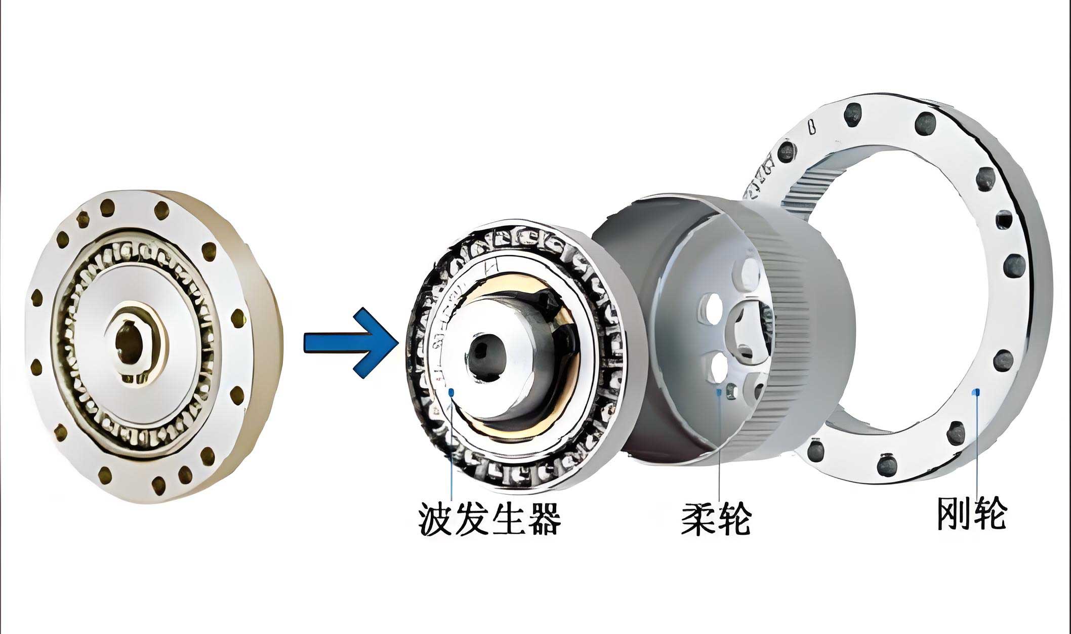
In my extensive work within the field of high-reliability mechanical design, particularly for aerospace applications, I have consistently encountered the critical challenge of performing accurate reliability assessments under significant data scarcity. Traditional methods often fall short, especially when initial design parameters are infused with subjective judgment or expert opinion alongside sparse objective data. This is profoundly evident in the analysis of critical spacecraft components like the strain wave gear. The strain wave gear, also known as a harmonic drive, is a cornerstone of precision motion control in satellites, found in solar array drive assemblies and antenna pointing mechanisms. Its advantages—high reduction ratios, compactness, near-zero backlash, and high torque capacity—are well-documented. However, its long-term reliability in the harsh space environment, where failure is not an option, remains a paramount concern. The conventional approach of assigning fixed values to lifetime model parameters is overly simplistic and can lead to dangerously optimistic or misleading conclusions. In this article, I will detail a robust framework for analyzing the reliability of a strain wave gear that simultaneously accounts for two fundamental types of uncertainty: aleatory (inherent randomness) and epistemic (subjective lack of knowledge). This leads to a probability-nonprobability hybrid model, offering a more realistic and informative reliability prediction in the form of an interval.
1. Foundations of Uncertainty Representation and Handling
Before delving into the specific model for the strain wave gear, it is essential to establish how different forms of uncertainty are mathematically represented and processed. A clear distinction must be made between aleatory and epistemic uncertainty.
1.1 Aleatory Uncertainty: The Probabilistic Framework
Aleatory uncertainty is irreducible, stemming from the inherent randomness of a phenomenon. It is appropriately modeled using probability theory. For parameters where sufficient test or historical data exists, a probability distribution function (PDF) can be fitted. Two key tools in this framework are crucial for our analysis.
Bayesian Estimation for Parameter Updating: Often, we have prior belief about a parameter (e.g., from handbook values or similar components) which can be combined with new, albeit limited, test data. Let a random parameter $\theta$ have a prior density $\pi(\theta)$. Given a set of observations $\mathbf{x}$ with likelihood function $p(\mathbf{x}|\theta)$, the posterior density—our updated belief about $\theta$—is given by:
$$\pi(\theta|\mathbf{x}) \propto p(\mathbf{x}|\theta) \pi(\theta)$$
For instance, if the prior for a mean coefficient is normal and we obtain a new expert estimate, we can derive a refined posterior mean. This is particularly useful for parameters like the application service factor ($K_A$) in gear life models.
First-Order Reliability Method (FORM) – A Brief Review: For a component with a performance function $G(\mathbf{X})$, where $\mathbf{X}$ is a vector of random variables, failure occurs when $G(\mathbf{X}) < 0$. The failure probability is:
$$P_f = \Pr[G(\mathbf{X}) < 0] = \int_{G(\mathbf{x})<0} f_{\mathbf{X}}(\mathbf{x}) d\mathbf{x}$$
FORM approximates this complex integral by:
- Transforming $\mathbf{X}$ to a standard normal space $\mathbf{U}$ via isoprobabilistic transformations (e.g., Rosenblatt or Nataf).
- Finding the Most Probable Point (MPP) $\mathbf{u}^*$ on the limit state $G(\mathbf{u})=0$, which is the point of minimum distance from the origin. This distance is the reliability index $\beta$.
- Approximating $P_f \approx \Phi(-\beta)$, where $\Phi$ is the standard normal CDF.
However, FORM requires gradient calculations and an iterative MPP search, which can be computationally expensive and non-robust for highly nonlinear or implicit functions. In the hybrid context with epistemic variables, this becomes a nested optimization, compounding the difficulty.
1.2 Epistemic Uncertainty: The Interval Framework
Epistemic uncertainty arises from a lack of knowledge. When data is extremely scarce, specifying a precise probability distribution is unjustified and potentially misleading. In such cases, an interval representation offers a prudent and less assumption-laden alternative. A variable $y$ with epistemic uncertainty is defined by its bounds: $y^I = [\underline{y}, \overline{y}] = \{y \in \mathbb{R} | \underline{y} \leq y \leq \overline{y}\}$.
When multiple, possibly conflicting, sources of information exist for an interval variable, they must be aggregated. Common operations include:
| Operation | Definition | Interpretation |
|---|---|---|
| Union | $y^I = [\min(y_i), \max(\overline{y}_i)]$ | Conservatively encompasses all possible ranges. |
| Average | $y^I = \left[ \frac{1}{n}\sum \underline{y}_i, \frac{1}{n}\sum \overline{y}_i \right]$ | Treats all sources as equally credible. |
| Weighted Mixture | $y^I = \left[ \sum w_i \underline{y}_i, \sum w_i \overline{y}_i \right], \sum w_i=1$ | Assigns different credibilities to sources. |
For a system whose safety is governed purely by interval variables $\mathbf{Y}$, a non-probabilistic reliability index $\eta$ can be defined based on the performance function $G(\mathbf{Y})$. Let $G^I = [\underline{G}, \overline{G}]$ be the interval of $G$. Defining the midpoint $G_c = (\underline{G}+\overline{G})/2$ and radius $G_r = (\overline{G}-\underline{G})/2$, the index is:
$$\eta = \frac{G_c}{G_r}$$
If $\eta > 1$, then $\underline{G} > 0$ and the system is reliably safe. If $\eta < -1$, then $\overline{G} < 0$ and the system is reliably failed. The interesting case is $-1 \leq \eta \leq 1$, where the sign of $G$ is uncertain, indicating a potentially unsafe state due to lack of knowledge.
2. The Probability-Nonprobability Hybrid Model for Strain Wave Gears
The reliability of a strain wave gear in a spacecraft is influenced by both types of uncertainty. Parameters like rated torque ($T_H$) and the service factor ($K_A$) may have enough manufacturing and test history to model probabilistically (aleatory). Conversely, operational parameters like the actual output torque ($T$) and input speed ($N_v$) during a mission are highly environment-dependent and may only be knowable within bounds (epistemic).
The standard life estimation model for a strain wave gear, where life is typically dictated by flexspline fatigue, is:
$$L_h = \left( \frac{3.575 \times 10^7}{N_v \cdot K_A} \cdot \frac{T_H}{T} \right)^3$$
where $L_h$ is the predicted life in hours. The associated performance function for a mission life of $m$ years (with 8,760 hours/year) is:
$$G(T_H, K_A, T, N_v, m) = L_h – 8760 \cdot m = \left( \frac{3.575 \times 10^7}{N_v K_A} \cdot \frac{T_H}{T} \right)^3 – 8760 m$$
Failure is defined as $G < 0$.
Now, let $\mathbf{X} = (T_H, K_A)$ be the random vector (aleatory) and $\mathbf{Y} = (T, N_v)$ be the interval vector (epistemic). The performance function becomes $G(\mathbf{X}, \mathbf{Y})$. For a fixed $\mathbf{Y}$, $G$ is a random variable, and we can compute a failure probability $P_f(\mathbf{Y})$. However, since $\mathbf{Y}$ can vary within its interval, $P_f$ itself becomes an interval: $P_f^I = [\underline{P_f}, \overline{P_f}]$.
To compute these bounds efficiently and robustly without nested MPP searches, I advocate for a response surface approach combined with interval analysis. The core idea is:
- Construct a Linear Approximate Limit State: Using a set of strategically sampled points (focusing on the region near $G \approx 0$), fit a linear hyperplane:
$$G(\mathbf{X}, \mathbf{Y}) \approx G_L(\mathbf{X}, \mathbf{Y}) = a_0 + a_1 T_H + a_2 K_A + a_3 T + a_4 N_v$$
This avoids the need for derivatives of the complex cubic function and is robust. - Compute Interval Bounds for Reliability Index: For the linear function $G_L$, with $\mathbf{X}$ being normal and $\mathbf{Y}$ interval, the reliability index $\beta$ becomes an interval $[\underline{\beta}, \overline{\beta}]$. The bounds are found by considering the combinations of interval endpoints that minimize or maximize $\beta$:
$$\underline{\beta} = \min_{\mathbf{Y} \in \mathbf{Y}^I} \frac{a_0 + a_1 \mu_{T_H} + a_2 \mu_{K_A} + a_3 T + a_4 N_v}{\sqrt{(a_1 \sigma_{T_H})^2 + (a_2 \sigma_{K_A})^2}}$$
$$\overline{\beta} = \max_{\mathbf{Y} \in \mathbf{Y}^I} \frac{a_0 + a_1 \mu_{T_H} + a_2 \mu_{K_A} + a_3 T + a_4 N_v}{\sqrt{(a_1 \sigma_{T_H})^2 + (a_2 \sigma_{K_A})^2}}$$
Given the monotonic nature of $G_L$ with respect to $T$ and $N_v$, the optima are typically at the vertices of the interval box for $\mathbf{Y}$. - Obtain Failure Probability Interval: The bounds of the failure probability are then:
$$\underline{P_f} = \Phi(-\overline{\beta}), \quad \overline{P_f} = \Phi(-\underline{\beta})$$
This result is profoundly informative. It doesn’t give a single, potentially deceptive number, but a range that quantifies how epistemic uncertainty propagates into the reliability metric. A wide interval $[\underline{P_f}, \overline{P_f}]$ signals a high sensitivity to lack of knowledge, guiding engineers to prioritize reducing epistemic uncertainty (e.g., via more testing or monitoring) for critical parameters.
3. Sensitivity Analysis within the Hybrid Framework
Sensitivity analysis reveals which parameters most influence the system’s reliability, guiding design improvements and risk mitigation strategies. In the hybrid model, we analyze sensitivity for both random and interval variables.
For a random variable $X_i$ with mean $\mu_i$ and standard deviation $\sigma_i$, the sensitivity of the average failure probability $\bar{P_f} = (\underline{P_f} + \overline{P_f})/2$ is derived. Using concepts from FORM sensitivity and averaging over the two limit states ($\underline{\beta}$ and $\overline{\beta}$), we get:
$$\frac{\partial \bar{P_f}}{\partial \mu_i} \approx -\frac{1}{2} \left[ \frac{\phi(\overline{\beta}) y_i^{*,(\overline{\beta})}}{\sigma_i \overline{\beta}} + \frac{\phi(\underline{\beta}) y_i^{*,(\underline{\beta})}}{\sigma_i \underline{\beta}} \right]$$
$$\frac{\partial \bar{P_f}}{\partial \sigma_i} \approx -\frac{1}{2} \left[ \frac{\phi(\overline{\beta}) (y_i^{*,(\overline{\beta})})^2}{\sigma_i \overline{\beta}} + \frac{\phi(\underline{\beta}) (y_i^{*,(\underline{\beta})})^2}{\sigma_i \underline{\beta}} \right]$$
where $\phi$ is the standard normal PDF, and $y_i^{*,(\cdot)}$ is the MPP coordinate in standard normal space for the respective limit state. A negative $\partial \bar{P_f}/\partial \mu_i$ indicates that increasing the mean of that variable reduces the average failure probability, making it a “strength” parameter.
For an interval variable $Y_j$, the sensitivity can be assessed via a finite-difference approach using the failure probability bounds:
$$\frac{\partial P_f}{\partial Y_j} \approx \frac{\Delta P_f}{\Delta Y_j} = \frac{P_f(Y_j=\overline{y}_j) – P_f(Y_j=\underline{y}_j)}{\overline{y}_j – \underline{y}_j}$$
This measures the rate of change of the failure probability interval’s width or location with respect to the variable’s range. A large absolute value indicates high epistemic importance.
4. Comprehensive Numerical Case Study: A Space-Borne Strain Wave Gear
Let us consider a strain wave gear unit designed for a satellite’s solar array drive. We define the parameters as follows:
| Variable | Description | Distribution | Mean ($\mu$) | Std. Dev. ($\sigma$) |
|---|---|---|---|---|
| $T_H$ | Rated Output Torque | Normal | 350 N·m | 35 N·m |
| $K_A$ | Service Factor | Normal | 1.3* | 0.1 |
*The mean of 1.3 for $K_A$ is derived via Bayesian updating of a prior $N(1.268, 0.08^2)$ with a new expert estimate of 1.35, following the principle $\pi(\mu_{K_A}|\text{data}) \propto p(\text{data}|\mu_{K_A}) \pi(\mu_{K_A})$.
| Variable | Source 1 | Source 2 | Aggregated Interval (Average) |
|---|---|---|---|
| $T$ (Output Torque) | [1900, 2150] N·m | [1900, 2080] N·m | [1900, 2115] N·m |
| $N_v$ (Input Speed) | [0.095, 0.112] rps | [0.085, 0.108] rps | [0.090, 0.110] rps |
The mission design life $m$ is varied from 10 to 15 years. Using the hybrid methodology described—fitting a linear approximation $G_L$ to the cubic life function near the failure boundary—we compute the interval failure probabilities. The results for the aggregated intervals are shown below.
| Design Life, $m$ (years) | Lower Bound, $\underline{P_f}$ | Upper Bound, $\overline{P_f}$ | Average, $\bar{P_f}$ | Reliability Interval $[1-\overline{P_f}, 1-\underline{P_f}]$ |
|---|---|---|---|---|
| 10 | 0.0082 | 0.1086 | 0.0584 | [0.8914, 0.9918] |
| 11 | 0.0151 | 0.1608 | 0.0880 | [0.8392, 0.9849] |
| 12 | 0.0253 | 0.2236 | 0.1245 | [0.7764, 0.9747] |
| 13 | 0.0386 | 0.2912 | 0.1649 | [0.7088, 0.9614] |
| 14 | 0.0575 | 0.3650 | 0.2113 | [0.6350, 0.9425] |
| 15 | 0.0793 | 0.4365 | 0.2579 | [0.5635, 0.9207] |
The results are striking. A deterministic analysis using midpoint values ($T=2007.5$ N·m, $N_v=0.1$ rps) would yield a single failure probability of approximately 0.156 for a 15-year life, suggesting a seemingly manageable risk. The hybrid model, however, reveals the profound impact of epistemic uncertainty: the actual failure probability could be as low as 0.079 or as high as 0.437. The system’s reliability for a 15-year mission is not a single value but lies somewhere between 56% and 92%. This interval quantifies the “lack-of-knowledge” risk. The widening interval with increased mission life clearly shows how epistemic uncertainty amplifies long-term prediction risk.
The sensitivity analysis for the 15-year mission yields the following insights:
| Parameter | $\partial \bar{P_f}/\partial \mu$ | $\partial \bar{P_f}/\partial \sigma$ | $\Delta P_f / \Delta Y$ (Interval) | Interpretation |
|---|---|---|---|---|
| $T_H$ (Rated Torque) | -5.53e-7 | 2.48e-8 | N/A | Increasing mean torque slightly improves reliability. Low sensitivity. |
| $K_A$ (Service Factor) | 0.047 | 0.445 | N/A | High positive sensitivity. Reducing $K_A$ (less severe service) greatly improves reliability. Uncertainty in $K_A$ ($\sigma$) is a major contributor. |
| $T$ (Output Torque) | N/A | N/A | ~0.0017 per N·m | Epistemic range strongly affects $P_f$ bounds. Lower operational torque is highly beneficial. |
| $N_v$ (Input Speed) | N/A | N/A | ~17.8 per rps | Extremely high epistemic sensitivity. Precise control/knowledge of input speed is the most critical factor for reliable life prediction. |
The sensitivity analysis conclusively identifies the input speed $N_v$ as the parameter demanding the most attention. Its massive epistemic sensitivity ($\Delta P_f / \Delta N_v \approx 17.8$) indicates that even small reductions in the uncertainty range of the operational speed (e.g., through better mission profiling or in-situ monitoring) would dramatically narrow the failure probability interval, leading to a more confident reliability assessment. This provides a clear directive for engineering resource allocation.
5. Discussion and Engineering Implications
The proposed hybrid framework for strain wave gear reliability analysis offers a pragmatic and robust advancement over traditional pure-probabilistic methods, especially in data-scarce, high-stakes environments like aerospace. By explicitly segregating and modeling aleatory and epistemic uncertainties, it provides a richer, more honest assessment. The output—a reliability or failure probability interval—directly communicates the confidence (or lack thereof) in the prediction.
This approach is particularly robust because it circumvents the need for nested optimization loops to find MPPs in a mixed variable space. The use of a locally accurate linear response surface, built from a focused set of samples, ensures computational efficiency and stability even with complex, implicit limit state functions.
For the practicing engineer designing or qualifying a strain wave gear for long-duration spaceflight, this methodology mandates a shift in thinking:
- Parameter Categorization: Consciously classify each input to the life model as either aleatory (fit a distribution) or epistemic (define an interval). This requires careful scrutiny of data sources.
- Informed Decision-Making: A single-point reliability figure is insufficient. Design decisions must consider the entire interval. A gear with a slightly worse midpoint reliability but a much narrower interval (less epistemic risk) might be preferable.
- Test Planning and Risk Reduction: The sensitivity analysis pinpoints which epistemic parameters contribute most to the prediction uncertainty. This justifies and prioritizes efforts to reduce those intervals through targeted testing, enhanced modeling, or system-level design changes (e.g., implementing torque limiters to narrow the $T$ interval).
The framework is not limited to strain wave gears. It is universally applicable to any reliability problem where data is incomplete and different forms of uncertainty coexist, such as in advanced materials, micro-electromechanical systems, or early-stage design of novel mechanical components. Embracing this interval-based probabilistic thinking is a crucial step towards more resilient and predictably reliable engineering systems.