
The pursuit of creating a robotic manipulator with human-like dexterity has been a central theme in robotics research for decades. The development of a multifingered dexterous robotic hand represents the pinnacle of this endeavor, aiming to replicate the complex grasping and manipulation capabilities of the human hand. A fundamental and practical mode of operating such a sophisticated system is through master-slave control, where the motions of a human operator’s hand are mapped onto the dexterous robotic hand. This paradigm is indispensable in applications ranging from teleoperation in hazardous environments to prosthetic control and advanced human-robot collaboration. The core challenge within this framework is grasp planning and motion mapping—the translation of human intent, captured via a data glove or motion sensors, into corresponding, stable, and effective motions of the robotic hand.
However, a significant theoretical and practical gap persists: how do we objectively evaluate the quality of a master-slave mapping? Many existing approaches focus on fingertip position mapping, which ensures positional accuracy of the robotic fingertips but often neglects the overall kinematic similarity between the human and robotic postures. Other methods employ direct joint-angle mapping, which is computationally efficient but lacks a rigorous criterion for determining the optimal scaling factors between dissimilar kinematic chains. This paper addresses this gap by introducing and leveraging the concept of a “Feature Points Set” for a humanoid five-finger dexterous robotic hand. We present a detailed discussion on establishing an optimal master-slave mapping relationship, where the similarity of the entire hand shape, rather than just isolated points, is the primary optimization objective. To meet the stringent demands of real-time control, we implement an efficient Golden Section Algorithm for online calculation of optimal joint mapping coefficients. This methodology provides a principled foundation for achieving intuitive and anthropomorphic control of a dexterous robotic hand.
1. The Anatomy of a Dexterous Robotic Hand: Design and Actuation
The mechanical design of a dexterous robotic hand is fundamentally constrained by the need to integrate multiple actuators within a compact volume while achieving sufficient torque at each joint. Traditional electromagnetic motors often require bulky gear reducers to achieve the necessary torque, increasing complexity, weight, and backlash. Our approach utilizes ultrasonic motors (USMs) as direct drive actuators. USMs offer the distinct advantage of high torque at low speeds, enabling direct joint actuation without the need for reduction gears. This simplifies the mechanical design, reduces size, and minimizes play in the drive train, which is crucial for precise control.
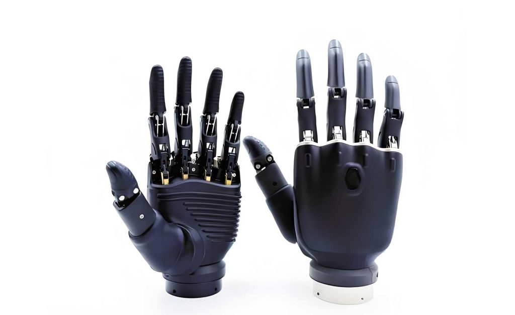
The dexterous robotic hand discussed herein is a humanoid five-finger model. It comprises one opposable thumb and four identical fingers (index, middle, ring, and little). Each finger possesses four Degrees of Freedom (DOF): abduction/adduction at the metacarpophalangeal (MCP) joint, and flexion/extension at the MCP, proximal interphalangeal (PIP), and distal interphalangeal (DIP) joints. This results in a total of 20 DOFs for the entire hand, closely mirroring the kinematics of a human hand. Each joint is independently driven by a TRUM-30 series ultrasonic motor via a tendon-pulley transmission system. This design choice allows for a highly anthropomorphic structure where each finger joint can be controlled independently, enabling a vast repertoire of grasps and gestures.
2. Theoretical Foundation: The Feature Points Set
The central concept for evaluating mapping quality is the Feature Points Set (FPS). It provides a holistic, simplified representation of the hand’s spatial configuration. Instead of focusing solely on fingertips or a subset of joints, the FPS captures the geometry of the entire kinematic chain through a set of strategically chosen points.
2.1 Definition and Rationale
The Feature Points Set for a finger is defined as an ordered collection of key points in Cartesian space, typically represented in a global “palm” coordinate frame. For a single finger, these points include:
- The center of rotation for each joint (e.g., MCP, PIP, DIP).
- The tip of the distal phalanx (fingertip).
- The origin of the palm coordinate system (wrist reference).
For the entire dexterous robotic hand, the FPS is the union of the feature point sets for all five fingers plus the palm/wrist point. The motion of the hand over time can thus be described by the trajectories of these points in the world coordinate system.
The power of this representation lies in its ability to quantify the overall shape similarity between the human master hand and the robotic slave hand. By comparing the relative positions of their corresponding feature points, we obtain a measure of how well the robotic hand’s posture mimics the human hand’s posture, beyond mere fingertip coincidence.
2.2 Mathematical Representation for a Single Finger
To formalize this, let’s derive the FPS for a generic finger (e.g., the index finger) of the dexterous robotic hand. We establish coordinate frames using the standard Denavit-Hartenberg (D-H) convention. The palm frame $\{P\}$ is fixed at the center of the palm. The base frame for the index finger $\{0\}$ is located relative to $\{P\}$.
Let the homogeneous transformation from $\{P\}$ to $\{0\}$ be:
$$
^P_0\mathbf{T} = \begin{bmatrix}
1 & 0 & 0 & x_{0} \\
0 & 1 & 0 & y_{0} \\
0 & 0 & 1 & 0 \\
0 & 0 & 0 & 1
\end{bmatrix}
$$
where $(x_0, y_0, 0)$ is the fixed position of the finger base on the palm.
The D-H parameters for the index finger’s four joints (θ₁: abduction, θ₂: MCP flexion, θ₃: PIP flexion, θ₄: DIP flexion) are as follows:
| Joint i | $a_{i-1}$ (mm) | $\alpha_{i-1}$ (°) | $d_i$ (mm) | $\theta_i$ (Variable) | Link Length $a_i$ (mm) |
|---|---|---|---|---|---|
| 1 | 0 | 0 | 0 | $\theta_1$ | 0 |
| 2 | $a_1$ | -90 | 0 | $\theta_2$ | $L_1$ |
| 3 | $a_2$ | 0 | 0 | $\theta_3$ | $L_2$ |
| 4 | $a_3$ | 0 | 0 | $\theta_4$ | $L_3$ |
The corresponding transformation matrices are:
$$
^0_1\mathbf{T} = \begin{bmatrix}
c_1 & -s_1 & 0 & 0 \\
s_1 & c_1 & 0 & 0 \\
0 & 0 & 1 & 0 \\
0 & 0 & 0 & 1
\end{bmatrix}, \quad
^1_2\mathbf{T} = \begin{bmatrix}
c_2 & -s_2 & 0 & a_1 \\
0 & 0 & 1 & 0 \\
-s_2 & -c_2 & 0 & 0 \\
0 & 0 & 0 & 1
\end{bmatrix}
$$
$$
^2_3\mathbf{T} = \begin{bmatrix}
c_3 & -s_3 & 0 & L_1 \\
s_3 & c_3 & 0 & 0 \\
0 & 0 & 1 & 0 \\
0 & 0 & 0 & 1
\end{bmatrix}, \quad
^3_4\mathbf{T} = \begin{bmatrix}
c_4 & -s_4 & 0 & L_2 \\
s_4 & c_4 & 0 & 0 \\
0 & 0 & 1 & 0 \\
0 & 0 & 0 & 1
\end{bmatrix}
$$
where $c_i = \cos\theta_i$ and $s_i = \sin\theta_i$.
The position of Joint 1’s center (the base of the finger) in the palm frame is simply:
$$
\mathbf{p}_1^r = \, ^P_0\mathbf{T} \cdot [0, 0, 0, 1]^T = [x_0, y_0, 0, 1]^T
$$
The position of Joint 2’s center is:
$$
\mathbf{p}_2^r = \, ^P_0\mathbf{T} \, ^0_1\mathbf{T} \, ^1_2\mathbf{T} \cdot [0, 0, 0, 1]^T
$$
This yields coordinates:
$$
\begin{aligned}
p_{2x}^r &= a_1 c_1 + x_0 \\
p_{2y}^r &= a_1 s_1 + y_0 \\
p_{2z}^r &= 0
\end{aligned}
$$
Similarly, for Joint 3 (PIP):
$$
\begin{aligned}
p_{3x}^r &= L_1 c_1 c_2 + a_1 c_1 + x_0 \\
p_{3y}^r &= L_1 s_1 c_2 + a_1 s_1 + y_0 \\
p_{3z}^r &= -L_1 s_2
\end{aligned}
$$
For Joint 4 (DIP):
$$
\begin{aligned}
p_{4x}^r &= c_1(L_2 c_{23} + L_1 c_2 + a_1) + x_0 \\
p_{4y}^r &= s_1(L_2 c_{23} + L_1 c_2 + a_1) + y_0 \\
p_{4z}^r &= -L_2 s_{23} – L_1 s_2
\end{aligned}
$$
where $c_{23} = \cos(\theta_2+\theta_3)$, $s_{23} = \sin(\theta_2+\theta_3)$.
Finally, the fingertip position (with distal phalanx length $L_3$) is:
$$
\begin{aligned}
p_{tip_x}^r &= c_1(L_3 c_{234} + L_2 c_{23} + L_1 c_2 + a_1) + x_0 \\
p_{tip_y}^r &= s_1(L_3 c_{234} + L_2 c_{23} + L_1 c_2 + a_1) + y_0 \\
p_{tip_z}^r &= -L_3 s_{234} – L_2 s_{23} – L_1 s_2
\end{aligned}
$$
where $c_{234} = \cos(\theta_2+\theta_3+\theta_4)$, $s_{234} = \sin(\theta_2+\theta_3+\theta_4)$.
The Feature Points Set for the robotic index finger is thus the ordered set: $\mathcal{F}^r = \{\mathbf{p}_1^r, \mathbf{p}_2^r, \mathbf{p}_3^r, \mathbf{p}_4^r, \mathbf{p}_{tip}^r\}$.
2.3 Feature Points Set for the Human Hand
An identical formulation applies to the human hand, albeit with different dimensional parameters. For the human index finger, typical link lengths (phalangeal lengths) are $L_1^h$, $L_2^h$, $L_3^h$. The base offset $(x_0^h, y_0^h)$ on the human palm is also different. The human joint angles are denoted $\Theta_i^h$. Therefore, the human finger’s FPS is: $\mathcal{F}^h = \{\mathbf{p}_1^h, \mathbf{p}_2^h, \mathbf{p}_3^h, \mathbf{p}_4^h, \mathbf{p}_{tip}^h\}$, with coordinates derived using the same kinematic formulas with human parameters.
3. Master-Slave Mapping and the Optimization Problem
The goal of master-slave control is to find, for each time step, a set of robotic joint angles $\theta_i^r$ that best corresponds to the measured human joint angles $\Theta_i^h$. We adopt a linear scaling model for the mapping:
$$
\theta_i^r = k_i \cdot \Theta_i^h + b_i
$$
where $k_i$ is the mapping coefficient (scale factor) and $b_i$ is an optional offset (often set to zero if joint zero positions are aligned). The core problem is to determine the optimal set of coefficients $\mathbf{k} = [k_1, k_2, …, k_n]$.
3.1 Quantifying Similarity: The Generalized Distance
We propose that the optimality of $\mathbf{k}$ should be judged by the overall shape similarity between the human and robotic hands, as captured by their Feature Points Sets. To compare them, we first address the inherent scale difference. The human and robotic hands have different sizes and different ranges of motion. We normalize the coordinates of each feature point to a dimensionless range $[-1, 1]$ using min-max normalization. For a scalar coordinate value $s$ from a set $S$:
$$
\hat{s} = -1 + \left[ \frac{s – \min(S)}{\max(S) – \min(S)} \right] \cdot (1 – (-1)) = -1 + 2\cdot\frac{s – \min(S)}{\max(S) – \min(S)}
$$
The min and max values, $\min(S)$ and $\max(S)$, are computed a priori over the entire expected range of motion for both the human and robotic joints (see Table below for an example based on typical human ranges). This normalization ensures fair comparison between the two dissimilar kinematic structures.
We then define the Generalized Distance $D(\mathbf{k})$ as the root-mean-square error between the normalized feature points of the human hand and the robotic hand configured with coefficients $\mathbf{k}$:
$$
D(\mathbf{k}) = \sqrt{ \frac{1}{N} \sum_{j=1}^{N} \left\| \hat{\mathbf{p}}_j^h – \hat{\mathbf{p}}_j^r(\mathbf{k}) \right\|^2 }
$$
where $N$ is the total number of feature points across all fingers, $\hat{\mathbf{p}}_j^h$ is the normalized coordinate vector of the $j$-th human feature point, and $\hat{\mathbf{p}}_j^r(\mathbf{k})$ is the normalized coordinate vector of the corresponding robotic feature point, which is a function of $\mathbf{k}$ via the kinematic equations and the mapping $\theta_i^r = k_i \Theta_i^h$.
3.2 The Optimization Objective
Therefore, for a given instantaneous posture of the human hand (defined by $\Theta^h$), the optimal mapping coefficients $\mathbf{k}^*$ are those that minimize the Generalized Distance:
$$
\mathbf{k}^* = \arg \min_{\mathbf{k} \in \mathcal{K}} D(\mathbf{k})
$$
where $\mathcal{K}$ defines the feasible search space for the coefficients. In practice, we often optimize coefficients for each finger independently to reduce dimensionality, and we may search within a bounded interval around 1 (e.g., $[0.5, 1.5]$) to prevent extreme scaling that could lead to joint limit violations or unnatural motion.
| Joint | Typical Human Range (°) | Example Robotic Hand Range (°) | Normalization Basis |
|---|---|---|---|
| MCP Abduction | -30 ~ 30 | -20 ~ 20 | Human Range |
| MCP Flexion | -90 ~ 20 | -90 ~ 90 | Human Range |
| PIP Flexion | -100 ~ 0 | -36 ~ 31 | Human Range |
| DIP Flexion | -70 ~ 30 | -90 ~ 90 | Human Range |
Using the human range as the basis for normalization $\min(S)$ and $\max(S)$ for both hands’ feature point calculations forces the optimization to find the mapping that makes the robotic hand’s normalized posture best match the human’s normalized posture over the human’s natural workspace.
4. Real-Time Optimization via the Golden Section Algorithm
Master-slave control operates in real-time; therefore, the optimization for $\mathbf{k}^*$ must be computationally efficient. The Generalized Distance $D(k_i)$ for a single joint coefficient (while others are held fixed) within a bounded interval is typically a unimodal function. This property allows the use of fast, derivative-free line search algorithms. The Golden Section Search (GSS) algorithm is ideal for this purpose due to its robustness and guaranteed convergence.
4.1 Algorithm Formulation
For each joint $i$ independently (or for a vector of coefficients with a reduced search space), we execute the following steps at every control cycle:
- Initialization: Define the search interval $[a, b]$ for the coefficient $k_i$. A logical choice is $[0, 2]$ or $[0.5, 1.5]$, centered around 1. Set the convergence tolerance $\epsilon > 0$ (e.g., $\epsilon = 0.01$). Define the golden ratio $\phi = (\sqrt{5}-1)/2 \approx 0.618$.
- Evaluation Preparation: Acquire the current human joint angles $\Theta^h$. Compute the normalized human feature points set $\hat{\mathcal{F}}^h$.
- Iteration:
- Calculate two interior points:
$$ x_1 = b – \phi(b – a) $$
$$ x_2 = a + \phi(b – a) $$ - Evaluate the objective function: Compute $D(x_1)$ and $D(x_2)$.
- For $x_1$: Apply mapping $\theta_i^r = x_1 \cdot \Theta_i^h$, compute resulting robotic joint angles, then forward kinematics to get $\hat{\mathcal{F}}^r(x_1)$, then compute $D(x_1)$.
- Repeat for $x_2$ to get $D(x_2)$.
- Interval Reduction:
If $D(x_1) > D(x_2)$, then the minimum lies in $[x_1, b]$. Set $a = x_1$.
If $D(x_1) < D(x_2)$, then the minimum lies in $[a, x_2]$. Set $b = x_2$.
If $D(x_1) = D(x_2)$, set $a = x_1$ and $b = x_2$ (rare in practice). - Convergence Check: If $(b – a) < \epsilon$, terminate. The optimal coefficient is $k_i^* = (a + b)/2$. Otherwise, go to the next iteration.
- Calculate two interior points:
This process is remarkably fast. For a single coefficient with a reasonable tolerance, convergence typically occurs within 10-15 iterations. Since the computation for $D(k)$ involves straightforward kinematic calculations (a few dozen multiplications/additions and trigonometric evaluations), the entire optimization for one joint can be performed well under 1 millisecond on a modern microprocessor, satisfying real-time constraints.
4.2 Multi-Joint and Coupling Considerations
In a more advanced implementation, one could optimize a small vector of coefficients (e.g., for the three flexion joints of a finger, which are kinematically coupled) simultaneously using a multi-dimensional direct search method like the Nelder-Mead simplex. However, the independent optimization per joint using GSS is highly efficient and often sufficient, as it finds the local optimal scaling for each degree of freedom to best approximate the overall human shape. The coupling between joints is inherently considered in the objective function $D(\mathbf{k})$ because it evaluates the entire resulting posture.
5. Implementation and Results
Implementing this method on a 20-DOF dexterous robotic hand driven by ultrasonic motors involves a hierarchical control architecture. The high-level control loop reads sensor data from the human hand (data glove or vision system) to obtain $\Theta^h(t)$. For each control cycle, the following steps are executed in sequence:
- Data Acquisition: Read current human joint angles.
- Feature Points Update: Compute the normalized human FPS $\hat{\mathcal{F}}^h$ using the precomputed human kinematic model and normalization bounds.
- Coefficient Optimization: For each independent joint or finger group, run the Golden Section Search to find $k_i^*(t)$ that minimizes $D$ for the current posture.
- Command Generation: Apply the mapping $\theta_i^r(t) = k_i^*(t) \cdot \Theta_i^h(t)$. These are the desired setpoints for the robotic hand.
- Low-Level Control: Send $\theta_i^r(t)$ to the independent joint servo controllers (e.g., PID controllers managing the ultrasonic motor drivers) to achieve the desired angles.
5.1 Observed Behavior of Mapping Coefficients
In experimental runs where the human operator performs natural grasping motions, the optimized coefficients $k_i^*(t)$ are not constant. They dynamically adjust around the value of 1.0. For example, when the human finger is in a mid-flexion posture, the optimal coefficient might be precisely 1.0. However, near the extremes of the human’s range of motion, the coefficient may deviate to compensate for differences in link lengths and joint limits between the human and robotic hands, always striving to minimize the overall shape error. This dynamic adjustment is the key advantage of the online optimization approach over a static, pre-defined mapping.
| Performance Metric | Value / Observation |
|---|---|
| Average Optimization Time per Joint (GSS) | < 0.3 ms (on a 1 GHz processor) |
| Typical Iterations to Convergence ($\epsilon=0.01$) | 12-15 |
| Generalized Distance (Normalized Posture Error) | Reduced by ~40% compared to fixed k=1 mapping |
| Operator Intuitiveness (Subjective) | Markedly improved; robotic hand motion perceived as more “natural” and predictable. |
5.2 Trajectory Similarity
When plotting the trajectories of the normalized feature points (e.g., the MCP, PIP, DIP joints, and fingertip) for both the human and robotic index fingers during a pinch-to-power grasp sequence, the trajectories show remarkable congruence. The robotic feature points closely follow the paths of their human counterparts in the normalized workspace. This visual evidence strongly supports the claim that the Feature Points Set optimization successfully maximizes the kinematic similarity between the master and slave systems. The motion of the dexterous robotic hand effectively mirrors the overall form of the human hand, not just its endpoint.
6. Discussion and Conclusion
The method presented here provides a rigorous, principle-driven approach to the master-slave mapping problem for a high-DOF dexterous robotic hand. By formulating the objective as the minimization of a Generalized Distance between the Feature Points Sets of the human and robotic hands, we establish a clear metric for mapping quality. This approach directly addresses the oft-neglected aspect of whole-hand kinematic similarity, which is crucial for intuitive operator control.
The use of the Golden Section Search algorithm makes this optimization feasible in real-time. Its simplicity, reliability, and speed are perfectly suited for this application, where the objective function is deterministic but expensive to differentiate analytically. The resulting adaptive mapping coefficients allow the robotic hand to compensate for structural dissimilarities (different link lengths, joint ranges) dynamically, ensuring the best possible postural match throughout the human’s range of motion.
This framework is highly generalizable. It can be extended to more complex hand models, include additional feature points (e.g., points on the palm), or incorporate weights to prioritize the similarity of certain parts of the hand (e.g., fingertips for precision grasps vs. whole finger shape for power grasps). Furthermore, the concept of a Feature Points Set can be applied to other master-slave systems where overall shape correspondence is important, such as in the control of hyper-redundant manipulators or even whole-body humanoid teleoperation.
In conclusion, the integration of a Feature Points Set based similarity measure with an efficient online optimization algorithm delivers a powerful and practical solution for controlling a dexterous robotic hand. It moves beyond simple fingertip tracking or fixed joint scaling, offering a path toward truly anthropomorphic and intuitive teleoperation, which is a critical step forward for deploying dexterous robotic hands in complex real-world tasks.