
In modern industrial automation, the precision of robotic systems is paramount, and at the heart of many industrial robots lies the rotary vector reducer, a critical component for motion control. As a researcher focused on mechanical transmission systems, I have dedicated significant effort to understanding and mitigating transmission errors in rotary vector reducers. This article presents a comprehensive study on the dynamic transmission error of rotary vector reducers, combining mathematical modeling, simulation analysis, and experimental validation. The goal is to provide insights into error sources and contribute to the enhancement of reducer performance. Throughout this work, the term “rotary vector reducer” will be emphasized to highlight its central role in precision engineering.
The rotary vector reducer, often abbreviated as RV reducer, is a closed transmission device known for its high torque capacity, compact structure, and excellent positioning accuracy. It integrates a planetary gear stage and a cycloidal gear stage, offering a high reduction ratio with minimal backlash. However, transmission errors arising from manufacturing tolerances, assembly misalignments, and dynamic loads can degrade its performance, leading to reduced accuracy in applications such as robotic arms. In this study, I aim to develop a dynamic model that accounts for factors like间隙, contact deformation, and负载 effects, which are often overlooked in static analyses. By leveraging simulation tools like ADAMS and validating with experimental data, I seek to establish a reliable framework for error prediction and reduction in rotary vector reducers.
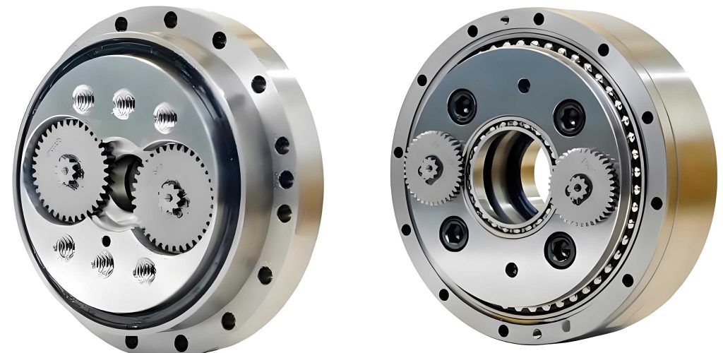
To begin, I will outline the fundamental structure and transmission principles of the rotary vector reducer. The device consists of an input shaft connected to a sun gear, which meshes with multiple planetary gears. These planetary gears are mounted on crankshafts that drive cycloidal gears (also known as摆线轮) engaging with a stationary pin gear housing. The output is taken from the planet carrier. The unique design of the rotary vector reducer allows for high reduction ratios, typically ranging from 30 to over 200, making it ideal for precision motion control. The transmission ratio is derived using the “fixed arm method” for planetary systems. For the planetary stage, the relationship between the sun gear and planetary gears is given by:
$$ i_{sp} = \frac{\omega_s – \omega_j}{\omega_p – \omega_j} = -\frac{z_p}{z_s} $$
where \( \omega_s \), \( \omega_p \), and \( \omega_j \) are the angular velocities of the sun gear, planetary gear, and planet carrier, respectively, and \( z_s \) and \( z_p \) are the tooth numbers. For the cycloidal stage, the transmission between the cycloidal gear and pin gear is:
$$ i_{wb} = \frac{\omega_b – \omega_p}{\omega_w – \omega_p} = -\frac{z_w}{z_b} $$
Here, \( z_b \) is the number of teeth on the cycloidal gear, and \( z_w = z_b + 1 \) is the number of pin teeth. Combining these, the overall transmission ratio of the rotary vector reducer, with the planet carrier as output, is:
$$ i_{sj} = 1 + \frac{z_p}{z_s} z_w $$
This formula underpins the high reduction capability of rotary vector reducers. In my analysis, I focus on a specific model, the SHPŔ-110E type rotary vector reducer, with material properties summarized in Table 1.
| Component | Material | Poisson’s Ratio | Moment of Inertia (kg·m²) | Elastic Modulus E (GPa) |
|---|---|---|---|---|
| Input Shaft | CrMo | 0.284 | 3.81 × 10⁻⁴ | 211 |
| Sun Gear | CrMo | 0.284 | 3.14 × 10⁻⁵ | 212 |
| Planetary Gear | CrMoAl | 0.277 | 8.05 × 10⁻⁴ | 212 |
| Crankshaft | GCr15 | 0.300 | 1.84 × 10⁻⁴ | 219 |
| Cycloidal Gear | CrMo | 0.292 | 2.89 × 10⁻² | 211 |
| Pin Gear Housing | GCr15 | 0.300 | 0.11 × 10⁻⁵ | 218 |
| Planet Carrier | GCr45 | 0.269 | 8.25 × 10⁻² | 210 |
Building on this foundation, I developed a dynamic mathematical model for the transmission error of the rotary vector reducer. The model employs the lumped mass method and dynamic substructure approach to represent the system as a set of interconnected masses and springs. Key interactions, such as gear meshing and bearing supports, are modeled using equivalent spring stiffnesses, as listed in Table 2.
| Interaction | Stiffness Symbol | Description |
|---|---|---|
| Sun Gear and Planetary Gear | \( k_{spi} \) | Meshing stiffness between sun and planetary gears |
| Sun Gear Support | \( k_s \) | Support stiffness for the sun gear |
| Planet Carrier and Pin Housing | \( k_{ca} \) | Connection stiffness between carrier and housing |
| Crankshaft and Cycloidal Gear | \( k_{dcji} \) | Stiffness at the crankshaft-cycloidal gear interface |
| Pin Tooth and Cycloidal Gear | \( k_{djk} \) | Meshing stiffness between pin teeth and cycloidal gear |
| Crankshaft and Planet Carrier | \( k_{bi} \) | Support stiffness for crankshafts on the carrier |
The dynamic equations are derived by considering forces and accelerations for each component. I established coordinate systems: a fixed frame at the pin gear center O, and moving frames attached to each cycloidal gear’s center \( O_j \) (for j=1,2), with axes aligned along eccentric directions. The equations account for displacements, eccentric errors, and间隙. For instance, the sun gear’s dynamics are described by:
$$ F_{sx} = k_s (X_s – E_{sa} \cos \beta_{sa}) $$
$$ F_{sy} = k_s (Y_s – E_{sa} \sin \beta_{sa}) $$
where \( F_{sx} \) and \( F_{sy} \) are support forces, \( X_s \) and \( Y_s \) are displacements, and \( (E_{sa}, \beta_{sa}) \) is the sun gear’s eccentric error. The meshing force between sun and planetary gears is:
$$ F_{spi} = k_{spi} \left( X_s \cos A_i + Y_s \sin A_i – X_{pi} \cos A_i – Y_{pi} \sin A_i – R_p (\theta_{pi} – \theta_p) + E_s \cos(\theta_s + \beta_{sa} – A_i) – E_{pi} \cos(\beta_{pi} – \theta_p – A_i) \right) $$
Here, \( A_i \) is the meshing line angle, \( R_p \) is the planetary gear radius, and \( E_{pi} \) is the planetary gear error. The equations of motion for the sun gear include centrifugal terms due to carrier rotation \( \omega_c \):
$$ m_s (\ddot{X}_s – 2\omega_c \dot{Y}_s – \omega_c^2 X_s) + F_{sx} + \sum_{i=1}^{3} F_{spi} \cos A_i = 0 $$
$$ m_s (\ddot{Y}_s + 2\omega_c \dot{X}_s – \omega_c^2 Y_s) + F_{sy} + \sum_{i=1}^{3} F_{spi} \sin A_i = 0 $$
$$ J_s \ddot{\theta}_s – R_s \sum_{i=1}^{3} (F_{spi} + F_{sp}) = 0 $$
Similar equations are derived for planetary gears, crankshafts, cycloidal gears, and the planet carrier, incorporating terms for contact deformations and间隙. For example, the force between crankshaft and cycloidal gear is modeled as:
$$ F_{dcjix} = k_{dcji} \left[ R_m (\theta_{doj} – \theta_{pi}) \sin(\theta_p + \psi_j) + X_{pi} – \eta_{dj} \cos(\theta_p + \psi_j) + R_{cd} (\theta_{dj} – \theta_c) \sin(\theta_{dj} – \theta_c) – E_{hji} \cos(\theta_c + \phi_i + \beta_{hji}) + E_{cji} \cos(\theta_p + \psi_j + \beta_{cji}) + \delta_c \right] $$
where \( R_m \) is the eccentric distance, \( \delta_c \) is the bearing clearance, and \( E_{hji} \) represents crankshaft hole errors. The planetary gear dynamics include:
$$ m_{sp} (\ddot{X}_{pi} – 2\omega_c \dot{Y}_{pi} – \omega_c^2 X_{pi}) – F_{spi} \cos A_i + \sum_{j=1}^{2} F_{dcjix} + F_{ccxi} = 0 $$
$$ m_{sp} (\ddot{Y}_{pi} + 2\omega_c \dot{X}_{pi} – \omega_c^2 Y_{pi}) + F_{spi} \sin A_i + \sum_{j=1}^{2} F_{dcjiy} + F_{ccyi} = -m_{sp} g $$
$$ J_{sp} \ddot{\theta}_{pi} – F_{spi} R_p – R_m \sum_{j=1}^{2} \left[ F_{dcjix} \sin(\theta_p + \psi_j) + F_{dcjiy} \cos(\theta_p + \psi_j) \right] = 0 $$
For cycloidal gears, the meshing force with pin teeth is:
$$ F_{dijs} = \delta_A k \left\{ \left[ R_m (\theta_{doj} – \theta_p) – R_d (\theta_{dj} – \theta_c) \right] \sin \alpha_{js} + \eta_{dj} \cos \alpha_{js} – P_{jk} \cos(\phi_{pdjs} – \alpha_{js}) – A_{Pjk} \sin(\phi_{pjs} – \alpha_{js}) – E_{Rk} \cos(\alpha_{js} – \phi_{Rjs}) – E_{A Rk} \sin(\alpha_{js} – \phi_{Rjs}) \right\} $$
where \( P_{jk} \) is the tooth profile deviation, and \( E_{Rk} \) is the pin tooth radial error. The equations of motion for cycloidal gears are:
$$ m_{bx} (\ddot{X}_{dj} – 2\omega_c \dot{Y}_{dj} – \omega_c^2 X_{dj}) + \sum_{i=1}^{3} P_{dcjix} + \sum_{i=1}^{Z_r} P_{dijs} \cos(\alpha_{js} + \theta_p + \psi_j) = 0 $$
$$ m_{bx} (\ddot{Y}_{dj} + 2\omega_c \dot{X}_{dj} – \omega_c^2 Y_{dj}) + \sum_{i=1}^{3} P_{dcjiy} + \sum_{i=1}^{Z_r} P_{dijs} \sin(\alpha_{js} + \theta_p + \psi_j) = m_{bx} g $$
$$ J_{oj} \ddot{\theta}_{dj} – \sum_{k=1}^{Z_r} (P_{dijs} + F_{dijs}) R_d \sin(\alpha_{js}) – R_{cd} \sum_{i=1}^{3} \left[ P_{dcjix} \sin(\theta_c + \phi_i) + P_{dcjiy} \cos(\theta_c + \phi_i) \right] = 0 $$
Finally, the planet carrier dynamics involve:
$$ F_{ccxi} = k_{bi} \left[ R_{dc} (\theta_{ca} – \theta_c) \sin(\theta_c + \phi_i) – X_{ca} + X_{pi} – E_{cai} \cos(\theta_c + \phi_i + \beta_{cai}) + \delta_{si} \right] $$
$$ F_{ccyi} = k_{bi} \left[ R_{dc} (\theta_{ca} – \theta_c) \cos(\theta_c + \phi_i) – Y_{ca} + Y_{pi} – E_{cai} \sin(\theta_c + \phi_i + \beta_{cai}) + \delta_{si} \right] $$
$$ F_{cax} = k_{ca} (X_{ca} – A_s \cos \beta_{ca} + \delta_{ca}) $$
$$ F_{cay} = k_{ca} (Y_{ca} – A_s \sin \beta_{ca} + \delta_{ca}) $$
and the equations of motion:
$$ m_{ca} (\ddot{X}_{ca} – 2\omega_c \dot{Y}_{ca} – \omega_c^2 X_{ca}) – F_{cax} + \sum_{i=1}^{3} F_{cxi} = 0 $$
$$ m_{ca} (\ddot{Y}_{ca} + 2\omega_c \dot{X}_{ca} – \omega_c^2 Y_{ca}) – F_{cay} – \sum_{i=1}^{3} F_{cyi} = -m_{ca} g $$
$$ J_{ca} \ddot{\theta}_{ca} – R_{dc} \sum_{i=1}^{3} \left[ F_{ccxi} \sin(\theta_c + \phi_i) + F_{ccyi} \cos(\theta_c + \phi_i) \right] = -T_{out} $$
These equations form a system of differential equations that I solved using the Newmark method in MATLAB. The transmission error \( \delta(t) \) is defined as the difference between the actual output angular displacement \( \theta_2(t) \) and the ideal output based on the input \( \theta_1(t) \) and reduction ratio \( i \):
$$ \delta(t) = \theta_2(t) – \frac{\theta_1(t)}{i} $$
For the rotary vector reducer with a ratio of 162, I computed the error over one output revolution. The results from the mathematical model show an error range of -35.9″ to 38.8″ (arcseconds), where positive values indicate lead errors and negative values indicate lag errors. The frequency spectrum reveals peaks at 260 Hz and 400 Hz, with amplitudes of 4.4″ and 0.62″, respectively. This analysis highlights the dynamic nature of errors in rotary vector reducers, influenced by factors like varying meshing stiffness and间隙.
To validate the mathematical model, I conducted a dynamic simulation using ADAMS software. I created a 3D assembly model of the rotary vector reducer and imported it into ADAMS, where I applied constraints and forces to replicate real-world conditions. The constraints included revolute joints for rotating parts and gear contacts for meshing interactions, as summarized in Table 3.
| Components | Constraint Type |
|---|---|
| Input Shaft and Ground | Revolute Joint |
| Input Shaft and Sun Gear | Gear Pair |
| Sun Gear and Planetary Gears | Contact Force |
| Planetary Gears and Crankshafts | Fixed Joint |
| Crankshafts and Cycloidal Gears | Revolute Joint |
| Cycloidal Gears and Pin Teeth | Impact Contact |
| Planet Carrier and Ground | Revolute Joint |
Contact forces were modeled using the impact function in ADAMS, which computes elastic and damping forces between colliding bodies. The function is defined as:
$$ \text{Impact} = \begin{cases}
k(q_1 – q)^e – c_{\text{max}} \dot{q} \cdot \text{step}(q, q_1 – d, 1, q_1, 0) & \text{if } q < q_1 \\
0 & \text{if } q \geq q_1
\end{cases} $$
where \( q \) is the distance between bodies, \( k \) is stiffness, \( e \) is the force exponent, \( c_{\text{max}} \) is damping, and \( d \) is the damping ramp-up distance. I set parameters based on material properties to ensure realistic contact behavior. For the simulation, I applied an input speed of 1600 rpm to the rotary vector reducer, corresponding to a theoretical output speed of 9.87 rpm for one revolution in 6 seconds. The simulation output speed was approximately 9.9 rpm, closely matching the expected value.
Using the simulation data, I calculated the transmission error in MATLAB via the Newmark method. The error curve from ADAMS simulation shows a range of -36.23″ to 38.72″, which aligns well with the mathematical model. The frequency spectrum also displays peaks at 260 Hz and 400 Hz, with amplitudes of 4.43″ and 0.62″, respectively. This consistency confirms the accuracy of my dynamic model for the rotary vector reducer. The slight variations may stem from simplifications in the mathematical model, such as linearized stiffness assumptions, whereas the ADAMS simulation incorporates nonlinear contact dynamics.
To further verify the findings, I designed and built an experimental platform for measuring transmission error in rotary vector reducers. The setup includes a drive motor, a rotary vector reducer under test, loading equipment, and measurement instruments. Optical encoders (圆光栅) are used to capture angular positions at the input and output shafts, with a magnetic powder brake applying负载 to simulate operating conditions. The platform ensures precise alignment and minimal external disturbances. I conducted tests on the SHPŔ-110E rotary vector reducer, applying an input speed of 1600 rpm and a负载 torque to replicate typical robotic applications. The transmission error was computed from the encoder data over multiple output revolutions to ensure statistical reliability.
The experimental results yield an error range of -36.1″ to 41.7″, which is slightly wider than the simulation results but still in close agreement. The frequency spectrum shows peaks at 260 Hz and 400 Hz, with amplitudes of 4.78″ and 0.65″, respectively. These values correlate well with both the mathematical model and ADAMS simulation, validating the overall approach. The minor discrepancies can be attributed to experimental uncertainties, such as encoder resolution, thermal effects, or unmodeled assembly tolerances in the actual rotary vector reducer. Nonetheless, the convergence of results across all three methods—mathematical modeling, simulation, and experiment—demonstrates the robustness of my analysis for rotary vector reducers.
In summary, this study provides a comprehensive framework for analyzing transmission error in rotary vector reducers. By developing a dynamic mathematical model that incorporates间隙, contact deformation, and负载 effects, I have captured key error sources often neglected in static analyses. The model was solved using the Newmark method, revealing error amplitudes within ±40 arcseconds for the tested rotary vector reducer. The ADAMS simulation corroborated these findings, with error curves and frequency spectra showing strong alignment. Experimental validation further confirmed the accuracy, with error ranges and spectral peaks consistent across all methods. This work underscores the importance of considering dynamic factors in the design and optimization of rotary vector reducers for high-precision applications. Future research could extend this approach to other reducer types or explore real-time error compensation techniques. Ultimately, enhancing the performance of rotary vector reducers will contribute to advancements in robotics and industrial automation, where precision and reliability are critical.
Throughout this article, I have emphasized the term “rotary vector reducer” to reinforce its significance in mechanical transmission systems. The integration of mathematical modeling, simulation, and experiment offers a holistic view of transmission error dynamics, paving the way for improved designs and reduced errors in rotary vector reducers. By addressing factors like variable stiffness and间隙, engineers can better predict and mitigate performance issues, leading to more accurate and efficient robotic systems. As technology evolves, the role of rotary vector reducers will only grow, making such analyses essential for future innovations.