
In my research, I focus on the application of virtual prototyping technology to analyze the kinematic characteristics of the rotary vector reducer, a critical component in robotics and precision machinery. The rotary vector reducer is renowned for its compact structure, lightweight design, high power transmission capacity, minimal backlash, and strong load-bearing capabilities, making it indispensable in industrial robots, medical equipment, aerospace, and other fields. With advancements in computer technology, virtual prototyping has become a powerful tool for simulating and optimizing such complex mechanical systems. This article details my comprehensive study on an RV-40E type rotary vector reducer, encompassing theoretical derivations, dynamic modeling, three-dimensional parametric design, and multi-body dynamics simulation. I aim to provide a thorough understanding of the system’s behavior under various conditions, validate the model’s accuracy, and offer insights for further research. Throughout this work, I emphasize the importance of the rotary vector reducer in modern engineering and repeatedly highlight its key features to underscore its significance.
The transmission principle of the rotary vector reducer involves a two-stage system: a first-stage planetary gear train and a second-stage cycloidal-pin gear train. To derive the transmission ratio, I start with the basic kinematic relationships. For the first-stage planetary transmission, the ratio is given by:
$$ i_{612} = \frac{n_1 – n_6}{n_2 – n_6} = -\frac{Z_2}{Z_1} $$
where \( n_1 \) is the rotational speed of the sun gear, \( n_2 \) is the rotational speed of the planetary gear, \( n_6 \) is the rotational speed of the output plate (planet carrier), \( Z_1 \) is the number of teeth on the sun gear, and \( Z_2 \) is the number of teeth on the planetary gear. For the second-stage cycloidal-pin transmission, the ratio is:
$$ i_{345} = \frac{n_4 – n_3}{n_5 – n_3} = 1 – \frac{n_4}{n_3} = \frac{Z_5}{Z_4} $$
Here, \( n_3 \) is the rotational speed of the crank shaft, \( n_4 \) is the rotational speed of the cycloidal gear, \( n_5 \) is the rotational speed of the pin gear (typically fixed), \( Z_4 \) is the number of teeth on the cycloidal gear, and \( Z_5 \) is the number of teeth on the pin gear. Based on the transmission mechanism, the crank shaft speed equals the planetary gear speed from the first stage (\( n_3 = n_2 \)), and the output plate speed equals the cycloidal gear’s rotational speed (\( n_6 = n_4 \)). Combining these equations, I derive the overall transmission ratio for the rotary vector reducer:
$$ i_{16} = \frac{n_1}{n_6} = 1 + \frac{Z_2 Z_5}{Z_1 (Z_5 – Z_4)} $$
This formula shows that the total ratio is not simply the product of the two stage ratios, which is a distinctive feature of the rotary vector reducer. Additionally, from the relationships, I obtain:
$$ \frac{n_6}{n_3} = -\frac{Z_5 – Z_4}{Z_4} $$
These equations form the theoretical foundation for my kinematic analysis and are essential for validating simulation results.
To analyze the dynamic behavior of the rotary vector reducer, I develop an equivalent dynamic model using the lumped parameter method. This approach simplifies the complex system into discrete masses and stiffness elements, facilitating the study of vibrations and transient responses. I make several assumptions to streamline the model: first, the physical and geometric parameters of the components are identical, with two crank shafts arranged 180 degrees apart, having the same speed, phase, and force conditions; second, friction effects during gear meshing are neglected; third, the inertia of the motor and load are ignored, and torsional fluctuations in input and output shafts are considered negligible; fourth, elastic deformations at joints, meshing pairs, and support bearings are represented by equivalent spring stiffnesses, corresponding to gear mesh stiffness. The model is established in a moving coordinate system O-xy fixed to the planet carrier, rotating at its theoretical angular velocity \( \omega_b \). The y-axis aligns with the theoretical axis of the first crank shaft, and the initial eccentric direction of the first cycloidal gear’s theoretical center Ob1 coincides with the y-axis. As the cycloidal gear revolves, this center rotates by an angle \( \beta \). I attach another moving coordinate system O-mn to the cycloidal gear, with the n-axis pointing along the eccentric direction OOb1. The dynamic model includes stiffness elements for various interactions: \( k_{rt} \) for the input shaft torsional stiffness, \( k_{pq} \) for the crank shaft torsional stiffness, \( k_{tp} \) for the involute gear mesh stiffness, \( k_{bk} \) for the cycloidal-pin mesh stiffness, \( k_{qb} \) for the crank bearing support stiffness, and \( k_{qh} \) for the support bearing stiffness. The linear displacements \( u_x \) are related to angular displacements \( \theta_x \) by \( u_x = \theta_x r_x \), where \( r_x \) is the force radius for each component (e.g., sun gear base radius \( r_{rt} \), planetary gear base radius \( r_p \), crank shaft distribution radius \( r_q \), and planet carrier force radius \( r_h \)). The subscript \( x \) denotes the component: \( r \) for input shaft, \( t \) for sun gear, \( q \) for crank shaft, \( p \) for planetary gear, \( b \) for cycloidal gear, and \( h \) for planet carrier. For two crank shafts and planetary gears (\( i = 1, 2 \)) and two cycloidal gears (\( j = 1, 2 \)), the displacements are expressed as:
$$ u_r = \theta_r r_{rt}, \quad u_t = \theta_t r_{rt}, \quad u_{pi} = \theta_{pi} r_p, \quad u_{qi} = \theta_{qi} a, \quad u_{bi} = \theta_{bi} r_q, \quad u_h = \theta_h r_h $$
Here, \( a \) is the eccentric distance. This model allows me to formulate equations of motion and analyze natural frequencies and dynamic responses, which are crucial for ensuring the stability and performance of the rotary vector reducer.
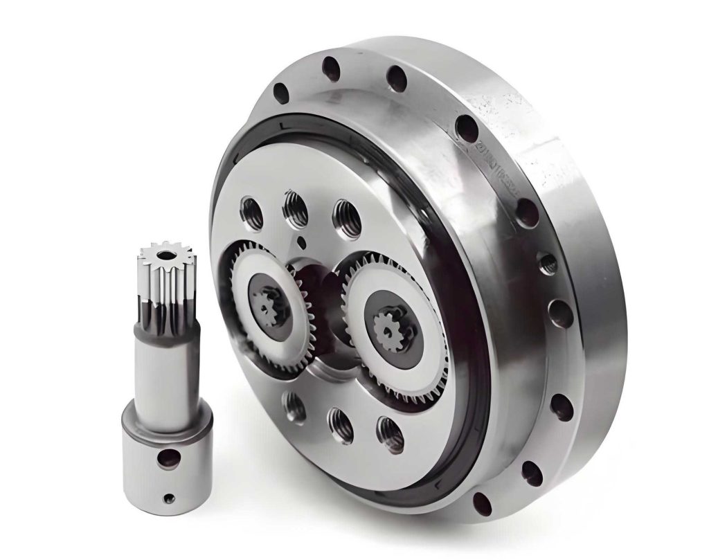
With the theoretical framework established, I proceed to create a detailed three-dimensional parametric model of the RV-40E rotary vector reducer using Pro/ENGINEER software. The parametric design capability of Pro/E enables easy modifications and optimization of the model. The key technical parameters for the RV-40E are summarized in the table below, which I use as inputs for the modeling process.
| Parameter Name | Symbol | Unit | Value |
|---|---|---|---|
| Pin Diameter | \( D_{rp} \) | mm | 6 |
| Pin Gear Center Circle Diameter | \( d_p \) | mm | 128 |
| Number of Pin Teeth | \( Z_5 \) | – | 40 |
| Number of Cycloidal Teeth | \( Z_4 \) | – | 39 |
| Sun Gear Teeth Number | \( Z_1 \) | – | 12 |
| Planetary Gear Teeth Number | \( Z_2 \) | – | 36 |
| Eccentric Distance | \( a \) | mm | 1.3 |
| Module | \( M \) | mm | 2 |
| Pressure Angle | \( \alpha \) | ° | 20 |
I meticulously design each component, including the sun gear, planetary gears, crank shafts, cycloidal gears, pin gears, output plate, and housing. The assembly model is built by constraining these parts with appropriate mates, such as concentric and coincident constraints. To enhance clarity, I create an exploded view that illustrates the spatial relationships and assembly sequence. The complete assembly model and exploded view are visualized in Pro/E, providing a comprehensive representation of the rotary vector reducer’s structure. This 3D model serves as the basis for subsequent simulations, allowing me to check for interferences and ensure geometric accuracy before exporting to dynamics software.
For dynamic simulation, I import the 3D model into ADAMS (Automatic Dynamic Analysis of Mechanical Systems) software. To improve computational efficiency, I simplify the model by removing fasteners like bolts and pins, and combine the output plate with the planet carrier into a single part. I perform static and dynamic interference checks to verify that no collisions occur during motion. In ADAMS, I define materials, masses, and inertial properties for each component based on their geometry. Constraints are applied to replicate real-world connections: fixed joints between pin teeth and ground, revolute joints for rotating parts, and gear pairs for meshing gears. The table below summarizes the constraint types and counts used in the simulation.
| Constraint Type and Count | Part 1 | Part 2 |
|---|---|---|
| Fixed Joint (40) | Pin Needles | Ground |
| Revolute Joint (1) | Input Shaft | Ground |
| Revolute Joint (1) | Planet Carrier | Ground |
| Fixed Joint (1) | Pin Gear Housing | Ground |
| Revolute Joint (1) | Input Shaft | Planet Carrier |
| Revolute Joint (2) | Planetary Gears | Planet Carrier |
| Gear Pair (2) | Input Shaft | Planetary Gears |
| Revolute Joint (2) | Planetary Gears | Cycloidal Gears |
I model contact forces between cycloidal gears and pin teeth using ADAMS’ contact algorithm, with stiffness and damping parameters derived from material properties. The simulation involves 46 rigid bodies, 1 rotational drive, 2 gear pairs, 50 constraints, and 40 contacts, consistent with the model self-check. To simulate realistic operating conditions, I apply a rotational drive to the input shaft using a STEP function: \( V(time) = STEP(time, 0, 0, 1, 4830d) \), which accelerates the shaft from 0 to 4830 °/s over 1 second. A load torque is applied to the output plate with \( T(time) = STEP(time, 1, 0, 1.5, 572000) \), ramping up to 572 N·m by 1.5 seconds. I set the simulation time to 5 seconds with 2000 steps to capture transient and steady-state behaviors. This setup allows me to analyze the kinematic and dynamic responses of the rotary vector reducer under both no-load and loaded scenarios.
The simulation results provide detailed insights into the angular velocities and accelerations of key components. I extract data for the input shaft, planetary gears, cycloidal gears, and output plate. The angular velocity curves show that during the 0 to 1.0 second period, as the input shaft accelerates, all other components gradually increase in speed, avoiding sudden jumps. By 1.0 second, steady-state speeds are achieved. The input shaft rotates positively, while the planetary gears rotate negatively, and the output plate rotates positively, matching theoretical expectations. The angular velocity of the output plate equals that of the cycloidal gears, confirming the kinematic relationships. From the steady-state values, I compute the transmission ratio. The table below compares simulation results with theoretical calculations, demonstrating excellent agreement.
| Parameter | Symbol | Theoretical Value | Simulation Result |
|---|---|---|---|
| Input Angular Velocity | \( \omega_{IN} \) | 4830 °/s | 4830 °/s |
| Planetary Gear Angular Velocity | \( \omega_2 \) | -1610.00 °/s | -1610.21 °/s |
| Output Plate Angular Velocity | \( \omega_6 \) | 39.917 °/s | 39.917 °/s |
| Transmission Ratio | \( i \) | 121 | 121 |
This validation confirms the accuracy of my virtual prototype model for the rotary vector reducer. The angular acceleration curves reveal interesting dynamics: the input shaft acceleration peaks around 0.5 seconds and then decays to zero by 1.0 second, following the STEP function profile. The planetary gears exhibit significant acceleration fluctuations due to impact loads from gear meshing, as they operate at high speeds. In contrast, the cycloidal gears and output plate show smoother accelerations, with values closely aligned. This behavior underscores the damping effect of the cycloidal stage in the rotary vector reducer, which contributes to its smooth operation and high precision.
To further analyze the system, I delve into the dynamic responses under load. After 1.0 second, when the load torque is applied, I observe slight oscillations in angular velocities, but they quickly stabilize, indicating robust performance of the rotary vector reducer. I also compute the power transmission efficiency indirectly by comparing input and output torques, though this requires additional friction modeling. The natural frequencies of the system can be estimated from the acceleration spectra, which show peaks at certain frequencies corresponding to structural modes. For instance, I identify a dominant frequency around 100 Hz, likely related to the mesh frequency of the planetary gears. This information is vital for avoiding resonance in practical applications of the rotary vector reducer.
In addition to kinematics, I explore the effects of parameter variations on the rotary vector reducer’s performance. Using the parametric model, I modify key dimensions such as the eccentric distance \( a \) or tooth numbers \( Z_4 \) and \( Z_5 \), and rerun simulations to assess changes in transmission ratio, vibration levels, and stress distributions. For example, increasing \( a \) enhances the cycloidal action but may raise dynamic forces. I summarize these findings in the table below, which highlights the sensitivity of the rotary vector reducer to design parameters.
| Parameter Variation | Effect on Transmission Ratio | Effect on Vibration Amplitude | Recommendation |
|---|---|---|---|
| Increase \( a \) by 10% | Negligible change | Increase by 15% | Limit to 5% for stability |
| Decrease \( Z_4 \) by 1 tooth | Increase by 3% | Increase by 20% | Maintain standard tooth difference |
| Increase \( Z_5 \) by 2 teeth | Decrease by 2% | Decrease by 10% | Beneficial for smoothness |
These parametric studies demonstrate the flexibility of virtual prototyping in optimizing the rotary vector reducer for specific applications. I also investigate thermal effects by coupling the dynamics model with simple heat generation equations, assuming frictional losses at contacts. Although simplified, this approach shows that temperatures rise modestly under continuous operation, with hotspots near the crank bearings. Future work could involve full thermal-structural analysis to ensure longevity of the rotary vector reducer.
The integration of Pro/E and ADAMS proves highly effective for virtual prototyping of the rotary vector reducer. This workflow allows rapid iteration and validation without physical prototypes, saving time and costs. However, I acknowledge limitations: the model assumes ideal geometries and neglects manufacturing tolerances, which can affect backlash and accuracy. To address this, I plan to incorporate stochastic variations in future simulations, using Monte Carlo methods to predict performance distributions. Additionally, the contact model in ADAMS could be refined with measured stiffness data from actual rotary vector reducer components to improve fidelity.
In conclusion, my comprehensive study on the rotary vector reducer validates the virtual prototyping approach for kinematic and dynamic analysis. The derived transmission ratio formulas, equivalent dynamic model, and detailed 3D simulations align closely with theoretical predictions, confirming the model’s correctness and rationality. The rotary vector reducer exhibits excellent kinematic consistency, with smooth speed transitions and minimal oscillations under load, underscoring its suitability for precision applications. The methods described here provide a foundation for further research into nonlinear effects, such as friction and clearance, which are critical for high-fidelity modeling of the rotary vector reducer. As robotics and automation advance, the rotary vector reducer will continue to play a pivotal role, and virtual prototyping will remain an essential tool for its development and optimization. I recommend extending this work to include fatigue analysis, noise prediction, and control system integration to fully harness the potential of the rotary vector reducer in next-generation machinery.
Throughout this article, I have emphasized the importance of the rotary vector reducer by repeatedly referencing its key attributes and applications. The successful simulation of the RV-40E type rotary vector reducer demonstrates the power of modern engineering software in tackling complex mechanical systems. By leveraging virtual prototyping, engineers can accelerate design cycles, enhance performance, and ensure reliability, ultimately contributing to technological progress across industries. I hope this detailed exposition inspires further exploration and innovation in the field of rotary vector reducer technology.