
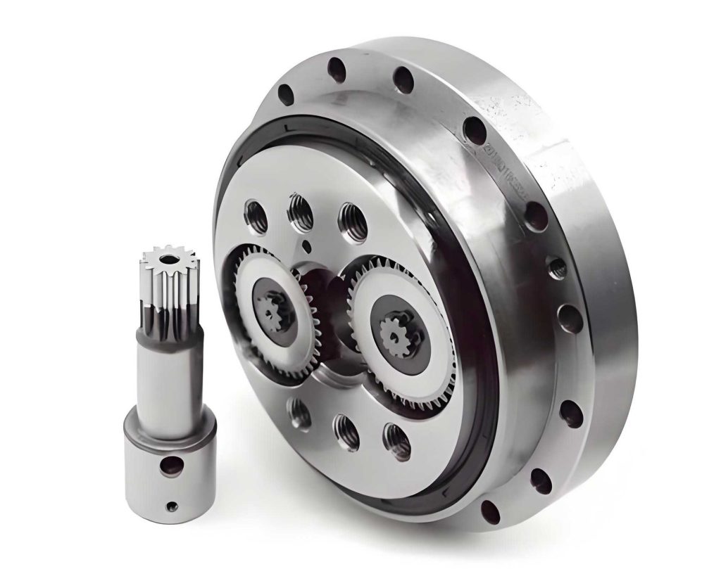
The manufacturing landscape, particularly in the domains of industrial robotics and automation, is witnessing a surge in demand for precision transmission components. Among these, the RV (Rotary Vector) reducer stands out as a critical, high-precision core component for industrial robots, enabling high torque, compact size, and exceptional positioning accuracy. However, achieving large-scale, efficient, and cost-effective production of RV reducers remains a significant challenge. The typical production strategy for a series of similar yet variant RV reducer models is the mixed-flow assembly line, which handles multiple product types on a single line. A primary bottleneck in such systems is line imbalance, where uneven distribution of work across stations leads to bottlenecks, underutilization, and overall efficiency loss. This imbalance directly impacts the production cycle time, smoothness of workflow, and ultimately, the scalability of production.
This article addresses the critical issue of production imbalance and low overall efficiency in RV reducer mixed-flow assembly lines. We establish a multi-objective mathematical model aimed at optimizing key performance indicators. To solve this model, we propose an enhanced Genetic Algorithm (GA) that incorporates a swap mutation operator considering precedence constraints to overcome the traditional GA’s tendency to converge prematurely to local optima. The effectiveness of the proposed methodology is then rigorously validated through discrete-event simulation using FlexSim software, demonstrating significant improvements in production metrics for an RV reducer assembly line.
Mathematical Model for Assembly Line Balancing
The fundamental problem in assembly line balancing is to assign a set of tasks (operations for assembling the RV reducer) to a sequence of workstations, obeying precedence constraints, to optimize one or more objectives. For a mixed-flow line producing multiple types of RV reducers, the model must account for the different processing times each product type requires for a given task.
Objective Functions
We consider three primary and interconnected objectives for optimizing the RV reducer assembly line:
1. Minimize Cycle Time ($$T_c$$): The cycle time is the maximum time taken by any workstation and dictates the pace of the entire line. Minimizing it increases throughput. It is defined as the maximum station time:
$$T_c = \max(T_1, T_2, …, T_K)$$
where $$T_k$$ is the total processing time assigned to workstation $$k$$, and $$K$$ is the total number of workstations.
2. Minimize Smoothness Index ($$S$$): This index measures the equity of workload distribution across stations. A lower value indicates a more balanced line, reducing work-in-process inventory and operator fatigue. It is calculated as:
$$S = \min \sqrt{\frac{\sum_{k=1}^{K}(T_c – T_k)^2}{K}}$$
3. Maximize Line Balance Rate ($$B$$): This is a direct measure of line efficiency, representing the ratio of total work content to the potential work content if all stations were as busy as the bottleneck station.
$$B = \frac{\sum_{i=1}^{K} T_i}{K \cdot \max(T_i)} \times 100\%$$
A perfect balance ($$B=100\%$$) means all station times are equal to the cycle time.
Constraints
The assignment of tasks to stations for the assembly of various RV reducer types must adhere to the following constraints:
Task Assignment Constraint: Each task (operation) for a specific product must be assigned to exactly one workstation.
$$\sum_{k=1}^{K} x_{i,k} = 1, \quad \forall i \in \text{Tasks}$$ where $$x_{i,k}=1$$ if task $$i$$ is assigned to station $$k$$.
Precedence Constraint: For any product, a task can only start at a station if all its immediate predecessor tasks have been completed. This is enforced by ensuring the start time of a task is later than the finish time of its predecessors.
Cycle Time Constraint: The total time of tasks assigned to any workstation $$k$$ for a specific product mix must not exceed the target cycle time $$T_c$$.
$$\sum_{i=1}^{N} (x_{i,k} \cdot t_{i,j}) \le T_c, \quad \forall k, \forall j$$ where $$t_{i,j}$$ is the time for task $$i$$ on product type $$j$$.
Station Occupancy Constraint: At any given time, a workstation processes only one product unit.
$$T_{i,j} \ge T_{i-1,j} + \sum_{k=1}^{K} x_{i,k} \cdot t_{i-1,j}, \quad \forall i,j$$
Improved Genetic Algorithm with Precedence-Considering Swap Mutation
Genetic Algorithms are well-suited for combinatorial optimization problems like assembly line balancing. However, standard GAs often struggle with constraint satisfaction (like precedence) and local convergence. We propose enhancements specifically for the RV reducer line balancing problem.
Chromosome Encoding and Initialization
A chromosome represents a potential solution—a sequence of all tasks for all RV reducer products in a production cycle. We use a precedence-based permutation encoding. For a line assembling multiple RV reducer types (e.g., Type A, B, C) in a certain ratio within a cycle, the chromosome is a list of task IDs (e.g., 1 to 40 for a cycle). The decoding process assigns tasks from this sequence to stations in order, respecting precedence relations and cycle time limits. The initial population is generated using a precedence-feasible random key method to ensure all initial solutions are valid.
Fitness Function
The fitness of a chromosome is a composite measure evaluating the three objectives. We primarily minimize cycle time and smoothness index. The fitness function $$F$$ can be defined as a weighted sum or a hierarchical evaluation. A typical formulation prioritizing cycle time is:
$$F = \frac{1}{(\alpha \cdot T_c + \beta \cdot S)}$$
where $$\alpha$$ and $$\beta$$ are weighting coefficients. Higher fitness indicates a better solution.
Genetic Operators
Selection: We employ a combination of elitism and tournament selection. The best few chromosomes (elites) are preserved to the next generation to prevent loss of good solutions. The rest of the population is filled by selecting parents through tournament selection, which promotes selection pressure towards fitter individuals.
Crossover: A precedence-preserving crossover operator, such as the Precedence Preservative Crossover (PPX), is used. PPX creates offspring by sequentially choosing tasks from two parent chromosomes based on a binary template string, ensuring the relative order of tasks (and thus precedence) is maintained from the parents.
Mutation – The Key Improvement: The standard mutation (random swapping of two tasks) often creates infeasible solutions by violating precedence. Our proposed Precedence-Considering Swap Mutation operates as follows:
- Randomly select a task $$i$$ from the chromosome.
- Identify the set of tasks that are not predecessors or successors of task $$i$$ (its “swap-feasible set”).
- Randomly select a second task $$j$$ from this swap-feasible set.
- Swap the positions of tasks $$i$$ and $$j$$ in the chromosome.
This operator introduces variability (exploration) while strictly adhering to the precedence constraints of the RV reducer assembly process, leading to a more efficient search through the feasible solution space.
Adaptive Parameter Control
To further avoid local optima, we implement adaptive crossover ($$P_c$$) and mutation ($$P_m$$) probabilities. Rates increase when population diversity is low (to encourage exploration) and decrease when good solutions are found (to encourage exploitation).
$$P_c = \begin{cases}
P_{c1} – \frac{(P_{c1}-P_{c2})(f’ – f_{avg})}{f_{max} – f_{avg}}, & f’ \ge f_{avg} \\
P_{c1}, & f’ < f_{avg}
\end{cases}$$
$$P_m = \begin{cases}
P_{m1} – \frac{(P_{m1}-P_{m2})(f_{max} – f)}{f_{max} – f_{avg}}, & f \ge f_{avg} \\
P_{m1}, & f < f_{avg}
\end{cases}$$
Here, $$f_{max}$$ and $$f_{avg}$$ are the maximum and average fitness in the current generation; $$f’$$ is the higher fitness of two parents for crossover; $$f$$ is the fitness of the chromosome to be mutated. This adaptive mechanism allows the algorithm to dynamically adjust its search strategy.
Algorithm Flow
The flowchart of the improved GA is summarized below:
- Initialize: Generate an initial population of precedence-feasible chromosomes. Set generation counter $$gen = 0$$.
- Evaluate: Decode each chromosome into a station assignment, calculate cycle time $$T_c$$, smoothness $$S$$, and fitness $$F$$.
- Termination Check: If $$gen \ge G_{max}$$ (max generations) or convergence criteria met, stop and output the best solution.
- Selection: Select parents using elitism and tournament selection.
- Crossover: Perform PPX crossover on selected parents with probability $$P_c$$ to produce offspring.
- Mutation: Apply the precedence-considering swap mutation to offspring with probability $$P_m$$.
- New Population: Form the next generation from elites and new offspring. Set $$gen = gen + 1$$, go to Step 2.
Case Study: Optimization of an RV Reducer Assembly Line
We applied the proposed model and algorithm to a real-world mixed-flow assembly line for RV reducers at a manufacturing facility. The line was initially configured with 18 workstations handling 31 distinct assembly operations for a family of RV reducer products.
Initial State Analysis
The standard task times for the various RV reducer types at each workstation were aggregated. The target daily output was 1,600 units over an 8-hour (28,800-second) shift. The theoretical required cycle time was:
$$T_{c}^{req} = \frac{28,800 \text{ seconds}}{1,600 \text{ units}} = 18 \text{ seconds}$$
The initial assignment of tasks to the 18 stations led to the following station times and performance metrics, as shown in the table below. The bottleneck station time was 17.9 seconds.
| Workstation | Assigned Tasks | Station Time (s) |
|---|---|---|
| 1 | 1, 2, 3, 4, 5 | 12.8 |
| 2 | 6, 7 | 13.2 |
| 3 | 8, 9 | 12.5 |
| 4 | 10, 11 | 11.4 |
| 5 | 12, 13 | 13.8 |
| 6 | 14 | 15.5 |
| 7 | 15 | 10.1 |
| 8 | 16, 17 | 11.1 |
| 9 | 18, 19, 20 | 15.6 |
| 10 | 21 | 9.6 |
| 11 | 22, 23 | 12.8 |
| 12 | 24 | 8.5 |
| 13 | 25, 26 | 13.7 |
| 14 | 27 | 12.9 |
| 15 | 28, 29 | 11.4 |
| 16 | 30 | 17.9 |
| 17 | 31 (Part 1) | 15.3 |
| 18 | 31 (Part 2) | 14.2 |
The initial performance was calculated as:
$$T_c^{initial} = 17.9 \text{ s}, \quad S^{initial} = 1.32, \quad B^{initial} = \frac{232.3}{18 \times 17.9} \times 100\% \approx 72\%$$
The low balance rate and high smoothness index confirmed significant imbalance.
Optimization via Improved GA
The improved GA was implemented with the following parameters: Population Size = 150, Maximum Generations ($$G_{max}$$) = 500, Adaptive $$P_{c1}=0.9, P_{c2}=0.6$$, Adaptive $$P_{m1}=0.1, P_{m2}=0.01$$. The algorithm was run to find an optimal task reassignment. The optimization revealed that the workload could be consolidated into 15 workstations while improving all metrics.
| Workstation | Assigned Tasks | Station Time (s) |
|---|---|---|
| 1 | 1, 2, 26, 3 | 16.3 |
| 2 | 5, 6 | 16.4 |
| 3 | 4, 8, 9 | 16.6 |
| 4 | 16, 27 | 16.5 |
| 5 | 15, 10 | 17.0 |
| 6 | 7, 13 | 15.2 |
| 7 | 11 | 15.5 |
| 8 | 14, 12 | 14.6 |
| 9 | 17, 19 | 15.6 |
| 10 | 20, 18, 21 | 15.3 |
| 11 | 22, 23 | 13.7 |
| 12 | 24 | 12.9 |
| 13 | 25, 28 | 17.2 |
| 14 | 29 | 15.3 |
| 15 | 30, 31 | 14.2 |
The optimized performance metrics are:
$$T_c^{opt} = 17.2 \text{ s}, \quad S^{opt} = 0.72, \quad B^{opt} = \frac{232.3}{15 \times 17.2} \times 100\% \approx 90\%$$
The results show a reduction in cycle time, a dramatic improvement in balance rate, and a much lower (better) smoothness index.
Simulation Validation with FlexSim
To validate the practical feasibility and dynamic performance of the optimized RV reducer line design, a detailed simulation model was built in FlexSim. The model accurately represented the 15 workstations, material flow, operators, and the processing times from the optimized schedule. The arrival of different RV reducer types followed the required production mix. The model was run for a simulated 8-hour shift.
Key Performance Output from FlexSim: The simulation confirmed the static calculations. The bottleneck station operated at close to 100% utilization, with an average cycle time of approximately 17.2 seconds. The dashboard analytics within FlexSim provided a station utilization pie chart, showing an average station utilization of 82.68%, with the highest at 91.82%. This demonstrated a significant reduction in idle time compared to the original line and confirmed the smooth, balanced flow of RV reducers through the system.
Summary of Improvements
| Performance Metric | Initial State | Optimized State | Improvement |
|---|---|---|---|
| Cycle Time ($$T_c$$) | 18.0 s | 17.2 s | Reduced by 0.8 s (4.4%) |
| Number of Workstations ($$K$$) | 18 | 15 | Reduced by 3 (16.7%) |
| Balance Rate ($$B$$) | 72% | 90% | Increased by 18 points |
| Smoothness Index ($$S$$) | 1.32 | 0.72 | Reduced by 0.60 (45.5%) |
Conclusion
The efficient and balanced production of RV reducers is paramount for meeting the growing demands of advanced manufacturing and robotics. This work presented a comprehensive methodology for optimizing mixed-flow assembly lines for RV reducers. By formulating a multi-objective mathematical model targeting cycle time, balance rate, and smoothness index, and subsequently solving it with an improved Genetic Algorithm—featuring a novel precedence-considering swap mutation and adaptive controls—we successfully addressed the classic line balancing problem with the specific constraints of RV reducer assembly.
The case study demonstrated the practical efficacy of the approach. The optimized line configuration reduced the number of workstations from 18 to 15 while simultaneously improving all key metrics: the production cycle time was shortened, the balance rate saw an 18-point increase, and the line smoothness was greatly enhanced. FlexSim simulation provided robust validation of the optimized design under dynamic conditions. This methodology offers a powerful tool for manufacturers of precision components like the RV reducer to systematically design, analyze, and optimize their production systems, thereby increasing throughput, reducing costs, and strengthening their competitive position in the market. The principles are also widely applicable to other complex, mixed-model assembly environments.