
The pursuit of reliable, high-precision motion drives the heart of modern automation. Within the intricate joints of industrial manipulators, surgical robots, and aerospace mechanisms, a compact yet powerful component performs a critical task: the Rotate Vector (RV) reducer. The RV reducer’s unique combination of high torque density, excellent torsional stiffness, and compact form factor has made it indispensable. However, its long-term reliability under the demanding, cyclical loads of real-world operation is paramount. Predicting and validating the lifespan of an RV reducer is therefore a fundamental challenge, bridging sophisticated theoretical analysis with rigorous physical validation. This article delves into the core of this challenge, presenting a comprehensive methodology for calculating the fatigue life of an RV reducer based on established strength theories and detailing a practical framework for accelerated life testing. This integrated approach, from fundamental models to validation protocols, provides a robust pathway for ensuring the durability and trustworthiness of these precision transmission systems.
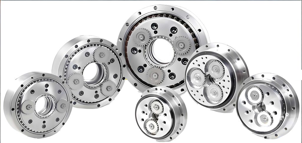
An RV reducer is not a simple gearbox; it is a planetary system that ingeniously combines a first-stage involute gear train with a second-stage cycloidal drive. This dual-stage design is the source of its high reduction ratio and exceptional load distribution capabilities. The output stage, featuring cycloidal discs meshing with stationary pins, is subjected to complex, multi-directional contact stresses. The crankshaft bearings, supporting the eccentric motion of the cycloidal discs, operate under particularly severe conditions of combined radial and cyclic loading. It is widely recognized that the fatigue life of these crankshaft bearings is often the limiting factor for the overall life of the RV reducer. Consequently, an accurate life prediction model must focus on the stress history and fatigue accumulation within these critical components.
The theoretical cornerstone for our RV reducer life calculation is the well-established concept of material fatigue. Cyclic loading below the ultimate tensile strength can still cause failure through the initiation and propagation of cracks. This phenomenon is governed by the material’s S-N (Stress vs. Number of cycles) curve, which defines the relationship between the stress amplitude ($\sigma_a$) and the number of cycles to failure ($N_f$) for a given material under specific conditions. The S-N relationship is typically expressed as a power law:
$$
\sigma_a^m \cdot N_f = C
$$
where $m$ is the fatigue strength exponent and $C$ is a material constant. Since the load on a crankshaft bearing in an RV reducer is directly proportional to the output torque ($T$), we can adapt this fundamental law to express life in terms of load:
$$
T^{m’} \cdot N_f = C’ \quad \text{or} \quad F^{m’} \cdot N_f = C”
$$
Here, $F$ represents the bearing load, and $m’$ is a load-life exponent derived from the system’s geometry and material properties.
In real-world operation, an RV reducer does not experience a single, constant load. A typical robotic duty cycle involves periods of acceleration, constant velocity, deceleration, and dwell, each associated with different torque levels. This variable loading scenario requires the application of a damage accumulation rule. The Palmgren-Miner linear damage accumulation hypothesis provides a practical and widely used framework. It posits that the total damage ($D$) from a sequence of varying stress levels is the sum of the fractional damages incurred at each level. If a component undergoes $M_i$ cycles at a stress level that would cause failure in $N_i$ cycles, its damage fraction is $M_i / N_i$. Failure is predicted to occur when the cumulative damage equals unity:
$$
D = \sum_{i=1}^{l} \frac{M_i}{N_i} = 1
$$
where $l$ is the number of distinct load levels. This principle allows us to construct a basic life model for the RV reducer under variable loading. By equating the damage from a complex load spectrum to that from a single, reference load ($F_k$ or $T_k$), we can calculate an equivalent life:
$$
N_k = \sum_{i=1}^{l} M_i \left( \frac{F_i}{F_k} \right)^{m’} \quad \text{or} \quad N_k = \sum_{i=1}^{l} M_i \left( \frac{T_i}{T_k} \right)^{m’}
$$
This equation forms the basic life model applicable to any component within the RV reducer subjected to variable loading, with the crankshaft bearing being the primary focus.
To move from a general model to a specific calculation for the RV reducer, we must determine the load-life exponent $m’$ and establish the precise relationship between output torque and bearing load. For rolling element bearings, the standard load-life relationship given by ISO and bearing manufacturers is the Lundberg-Palmgren theory, which uses an exponent of $p=10/3$ for roller bearings and $p=3$ for ball bearings. As the crankshaft bearings in most RV reducers are needle or cylindrical roller bearings, we adopt $m’ = p = 10/3$. The next step is force analysis. A detailed static force analysis of the cycloidal stage reveals that the load on each crankshaft bearing ($F$) varies periodically with the rotation of the crankshaft (angle $\theta$) and is a function of the output torque ($T$) and the RV reducer’s geometric parameters (eccentricity $e$, number of pins $Z_p$, pitch radius $R_p$, crank circle radius $r_0$, etc.).
The relationship can be derived as:
$$
F(\theta) = \frac{T}{2 \lambda e Z_c r_0} \cdot \sqrt{(e Z_c)^2 + (1+k_y^2)r_0^2 + 2 e Z_c r_0 (\cos\theta – k_y \sin\theta)}
$$
where $\lambda$ is the number of crankshafts (typically 2 or 3), $Z_c$ is the number of cycloid gear teeth ($Z_c = Z_p – 1$), and $k_y$ is a load distribution factor. This equation confirms that bearing load is directly proportional to output torque. Since the load varies, the equivalent dynamic load ($F_m$) for life calculation is found using the $p$-norm (with $p=10/3$ for roller bearings):
$$
F_m = \left( \frac{1}{2\pi} \int_0^{2\pi} [F(\theta)]^{10/3} d\theta \right)^{3/10}
$$
For a given RV reducer design, this integral yields a constant coefficient $K$ such that:
$$
F_m = K \cdot T
$$
This is a critical result: the equivalent bearing load for fatigue life calculation is a linear function of the output torque on the RV reducer.
| Parameter | Symbol | Value (Example RV-80E) |
|---|---|---|
| Eccentricity | $e$ | 1.45 mm |
| Pin Radius | $R_p$ | 76.5 mm |
| Number of Pins | $Z_p$ | 40 |
| Number of Cycloid Teeth | $Z_c$ | 39 |
| Crank Circle Radius | $r_0$ | 42 mm |
| Number of Crankshafts | $\lambda$ | 3 |
| Load Proportionality Constant | $K$ | 5.58 N/(N·m) (Calculated) |
The basic rating life ($L_{10}$) of a rolling bearing in hours, according to ISO 281, is calculated using the basic dynamic load rating ($C_d$) of the bearing and the equivalent dynamic load ($F_m$):
$$
L_{10} = \frac{10^6}{60 n} \left( \frac{C_d}{F_m} \right)^p
$$
where $n$ is the rotational speed in revolutions per minute (rpm). For the RV reducer’s crankshaft bearing, the speed $n$ is the rotational speed of the crankshaft relative to the cycloid disc. This is the input speed multiplied by the first-stage planetary ratio ($n’$). Substituting $F_m = K T$ and $p=10/3$, the rated life of the RV reducer at its rated torque ($T_0$) and rated input speed ($n’_0$) becomes:
$$
L_0 = \frac{10^6}{60 n’_0} \left( \frac{C_d}{K T_0} \right)^{10/3}
$$
This equation provides the theoretical $L_{10}$ life under constant rated conditions, where $L_{10}$ is defined as the life that 90% of a group of identical bearings will exceed.
Real-world operation is far from constant. To calculate the service life, we must account for the full duty cycle. Using the Palmgren-Miner rule and our adapted load-life relationship, we derive an equivalent torque ($T_m$) and equivalent speed ($n’_m$) for the variable condition. The service life ($L$) is then:
$$
L = \frac{10^6}{60 n’_m} \left( \frac{C_d}{K T_m} \right)^{10/3}
$$
The equivalent torque and speed can be calculated from a load spectrum. If the duty cycle consists of periods $t_i$ with torque $T_i$ and crankshaft speed $n’_i$, they are determined as:
$$
T_m = \left( \frac{\sum (t_i \cdot n’_i \cdot T_i^{10/3})}{\sum (t_i \cdot n’_i)} \right)^{3/10}, \quad n’_m = \frac{\sum (t_i \cdot n’_i)}{\sum t_i}
$$
This formalism elegantly links the complex operational profile of the RV reducer to a single, equivalent constant-load scenario for life prediction. It clearly shows that increasing either the equivalent torque or the equivalent speed will reduce the predicted service life, which is the foundational principle for designing accelerated life tests.
Accelerated Life Testing (ALT) is essential for validating the theoretical life models of an RV reducer within a reasonable timeframe. The objective is to induce fatigue failure much faster than under normal use, while ensuring the failure modes remain representative. Based on the life equations, acceleration is achieved by increasing the load ($T_m$) and/or the speed ($n’_m$). The Acceleration Factor (AF) comparing test conditions (subscript $a$) to rated conditions is:
$$
AF = \frac{L_0}{L_a} = \frac{n’_a}{n’_0} \left( \frac{T_a}{T_0} \right)^{10/3}
$$
The exponent of $10/3$ underscores that increasing torque is significantly more effective for acceleration than increasing speed. Therefore, a high-torque, back-and-forth oscillatory motion is a common and effective test regimen.
Designing a valid ALT requires a loading profile that mimics realistic robot motion patterns, including acceleration and deceleration phases. A simple trapezoidal velocity profile creates discontinuous jerk (rate of change of acceleration), which induces unrealistic shock loads. A superior approach is to use an S-curve acceleration profile, which smoothly ramps acceleration up and down. This seven-phase profile (jerk+, acceleration+, jerk-, constant velocity, jerk-, acceleration-, jerk+) closely replicates the smooth motion of a well-tuned industrial robot. The motion parameters for one half-cycle (e.g., 180-degree swing) can be defined as shown in the table below:
| Phase | Duration $\Delta t$ (s) | Angular Acceleration $\alpha$ (rad/s²) | Angular Velocity $\omega$ (rad/s) |
|---|---|---|---|
| Jerk+ / Acceleration+ | $t_1$ | Ramps from 0 to $\alpha_{max}$ | $\omega = \frac{1}{2}j t^2$ |
| Constant Acceleration | $t_2$ | $\alpha_{max}$ | $\omega = \omega_1 + \alpha_{max} t$ |
| Jerk- / Acceleration- | $t_3$ | Ramps from $\alpha_{max}$ to 0 | $\omega = \omega_2 – \frac{1}{2}j t^2$ |
| Constant Velocity | $t_4$ | 0 | $\omega_{max}$ |
| Jerk- / Deceleration- | $t_5$ | Ramps from 0 to $-\alpha_{max}$ | $\omega = \omega_{max} – \frac{1}{2}j t^2$ |
| Constant Deceleration | $t_6$ | $-\alpha_{max}$ | $\omega = \omega_5 – \alpha_{max} t$ |
| Jerk+ / Deceleration+ | $t_7$ | Ramps from $-\alpha_{max}$ to 0 | $\omega = \omega_6 + \frac{1}{2}j t^2$ |
During testing, the RV reducer output shaft is connected to a load arm. The total torque ($T_{total}$) on the RV reducer is the sum of the inertial torque ($T_{inertial}$) from accelerating/decelerating the load’s moment of inertia ($J$), and the gravitational torque ($T_{gravity}$) from the weight of the load arm ($mg$) at different swing angles ($\phi$).
$$
T_{total} = T_{inertial} + T_{gravity} = J \cdot \alpha + m g l \cos(\phi)
$$
where $l$ is the distance from the pivot to the center of mass. The maximum torque typically occurs during the deceleration phase when gravity and inertia act in the same direction. By selecting an appropriate load arm mass and length, and defining the S-curve motion profile, we can precisely set the peak test torque ($T_a$) and calculate the equivalent test torque ($T_{m, test}$) and speed ($n’_{m, test}$) for the duty cycle. Substituting these into the service life equation yields a theoretical accelerated life duration for the test.
A standard ALT setup consists of a rigid base, a servo motor to drive the RV reducer input, a load arm attached to the output, and comprehensive monitoring systems. The motion controller executes the pre-defined S-curve oscillation profile. Key performance indicators are monitored throughout the test, with repeatability (or backlash) being one of the most sensitive to incipient wear and fatigue damage. A high-resolution displacement or angular sensor measures the output position at a fixed command point (e.g., at the end of each swing). As the internal components of the RV reducer, particularly the crankshaft bearings, begin to degrade, the scatter or drift in this positional data will increase, signaling the onset of failure.
Using the methodology outlined, consider an example for an RV-80E-type reducer with a rated torque $T_0 = 784$ Nm and a calculated rated life $L_0 = 6,000$ hours. For the ALT, we set the peak test torque $T_a = 2.5 \times T_0 = 1960$ Nm. Assuming the S-curve profile results in an equivalent test torque $T_{m,test} \approx 2.2 \times T_0$ and an equivalent speed factor, the acceleration factor can be calculated:
$$
AF = \left( \frac{T_{m,test}}{T_0} \right)^{10/3} \approx (2.2)^{10/3} \approx 20.7
$$
The predicted accelerated test life is therefore:
$$
L_{a, predicted} = \frac{L_0}{AF} = \frac{6000}{20.7} \approx 290 \text{ hours}
$$
A well-instrumented test would run until a predefined failure criterion is met, such as a doubling of the positional repeatability error or a significant change in vibration or temperature signature. A test result of, for example, 310 hours to failure would show excellent correlation with the theoretical prediction, validating the underlying fatigue life calculation model for the RV reducer.
| Description | Symbol | Value |
|---|---|---|
| Rated Life (Theoretical) | $L_0$ | 6,000 hours |
| Test Peak Torque | $T_a$ | 1,960 Nm (2.5 x $T_0$) |
| Test Equivalent Torque | $T_{m,test}$ | ~1,725 Nm (Calculated from duty cycle) |
| Calculated Acceleration Factor | $AF$ | ~20.7 |
| Predicted Test Life | $L_{a, predicted}$ | ~290 hours |
| Hypothetical Actual Test Life | $L_{a, actual}$ | 310 hours |
| Model Accuracy (Error) | – | ~6.3% |
The journey from fundamental fatigue strength theory to a validated accelerated test protocol provides a powerful and cohesive framework for mastering RV reducer life. By anchoring the analysis in the physics of rolling contact fatigue and the Palmgren-Miner cumulative damage rule, we can develop precise mathematical models for both rated and service life. The identification of the crankshaft bearing as the life-limiting component allows for targeted analysis. The derived life equations clearly quantify the profound impact of load, enabling the design of efficient accelerated life tests. Implementing these tests with motion profiles that reflect real-world robot dynamics, such as S-curve trajectories, ensures the validity of the failure modes observed. Ultimately, this integrated approach—combining rigorous calculation with representative physical testing—enables designers and engineers to predict, verify, and enhance the durability of the critical RV reducer, thereby bolstering the reliability and longevity of the advanced robotic systems that depend on them.