
In modern manufacturing systems, industrial robots serve as critical execution units, with the RV reducer being a core component due to its high torque capacity and precision. However, the operational health of the RV reducer is often compromised by factors such as variable speeds and heavy loads, making fault diagnosis challenging, especially when the input rotating speed is unknown or difficult to measure directly. Traditional methods rely on predefined speed parameters, which are impractical in dynamic industrial environments where robots undergo acceleration, constant velocity, and deceleration phases. This paper addresses this issue by proposing a novel fault diagnosis approach that leverages current and vibration signals from the RV reducer. By estimating instantaneous frequency from current signals, we derive the input rotation frequency and subsequently calculate fault characteristic frequencies for various components of the RV reducer. Vibration signals during steady-state operation are then analyzed using an adaptive variational mode decomposition algorithm optimized via particle swarm optimization. A multidimensional evaluation function is employed to select fault-sensitive components, followed by envelope analysis to extract fault features. This method enables effective health assessment of the RV reducer without prior knowledge of the rotating speed, enhancing reliability and accuracy in industrial applications. The RV reducer, with its complex gear system including planetary gears, cycloid gears, and needle bearings, is prone to wear and pitting, leading to performance degradation. Our approach integrates signal processing techniques to overcome these challenges, providing a robust solution for condition monitoring. In this work, we detail the methodology, experimental validation, and results, emphasizing the adaptability of the method to real-world scenarios. The RV reducer’s role in industrial robots underscores the importance of this research, as failures can cause operational downtime and costly repairs. By focusing on unknown speed conditions, we contribute to advancing predictive maintenance strategies for smart manufacturing.
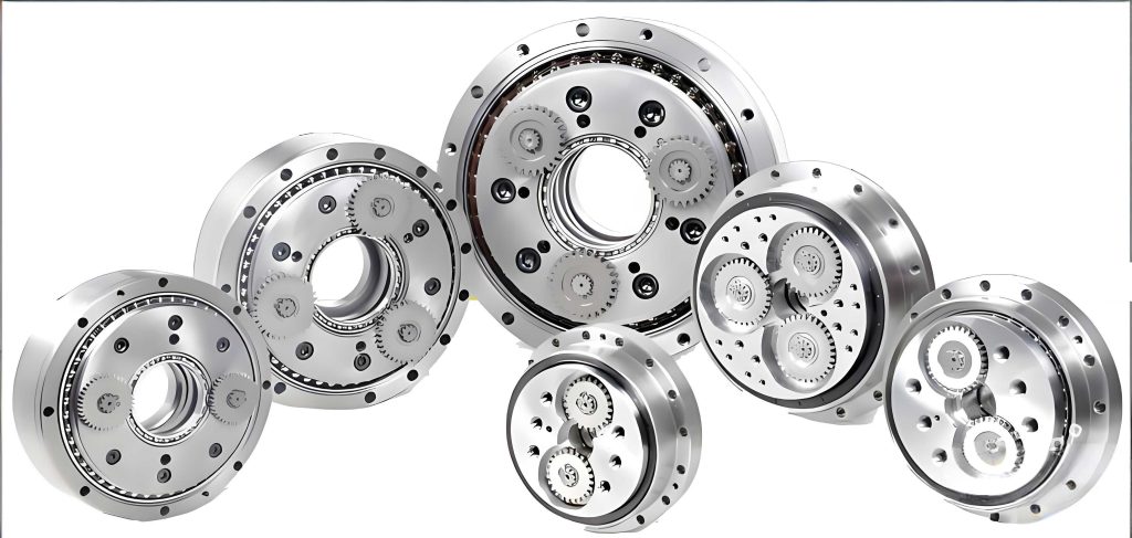
The RV reducer, a type of precision gearbox, is integral to industrial robot joints, transmitting motion from the motor to the linkage with high reduction ratios. Its structure typically involves a two-stage system: a planetary gear stage and a cycloid pin gear stage, which together provide high stiffness and torque. Faults in the RV reducer, such as gear tooth damage or bearing wear, manifest as vibrations and current fluctuations, but diagnosing these under variable speeds requires sophisticated signal analysis. In this paper, we introduce a hybrid approach that combines current-based speed estimation with vibration-based feature extraction. The current signal from the motor drive is analyzed using linear chirplet wavelet transform to estimate the instantaneous frequency, which corresponds to the motor’s electrical frequency. From this, the mechanical rotation frequency of the RV reducer input is derived, allowing computation of fault characteristic frequencies for components like the sun gear, planetary gears, and cycloid gears. Simultaneously, vibration signals from the RV reducer housing are captured during steady-speed intervals, processed through variational mode decomposition with parameters optimized by particle swarm optimization. This decomposition yields intrinsic mode functions, from which the most informative component is selected using a multidimensional evaluation function based on kurtosis, envelope spectrum kurtosis, and envelope entropy. Envelope analysis of this component then reveals fault-related frequency components, enabling diagnosis. The RV reducer’s health is thus assessed without direct speed measurement, addressing a key limitation in industrial settings. This method is validated through experiments on an RV reducer test rig, demonstrating its efficacy in detecting faults such as pitting in gears. The RV reducer’s complexity necessitates such advanced techniques, and our work provides a practical framework for implementation. Throughout this paper, we will elaborate on each step, supported by mathematical formulations and experimental data, to illustrate the method’s robustness.
To begin, let us formalize the signal acquisition process. We denote the vibration signal as $x(t) \in \mathbb{R}^{n \times 1}$ and the current signal as $s(t) \in \mathbb{R}^{n \times 1}$, where $n = T f_s$, with $T$ being the sampling duration and $f_s$ the sampling frequency. The current signal is first transformed into an analytical signal $z(t)$ using the Hilbert transform: $z(t) = s(t) + j \mathcal{H}[s(t)]$, where $\mathcal{H}[\cdot]$ represents the Hilbert operator. This analytical signal is then processed using the linear chirplet wavelet transform to obtain a time-frequency representation. The window function for this transform is defined as:
$$\psi(t, t_0, \alpha, \sigma) = w_{\sigma}(t – t_0) \exp\left(-j \frac{\alpha}{2} (t – t_0)^2\right),$$
where $t_0$ is the time center, $\alpha$ is the chirp rate, and $w_{\sigma}(t) = \frac{1}{\sqrt{2\pi}\sigma} \exp\left(-\frac{1}{2} \left(\frac{t}{\sigma}\right)^2\right)$ is a Gaussian window with width $\sigma$. The time-frequency matrix $TF(t_0, \omega, \alpha, \sigma)$ is computed as:
$$TF(t_0, \omega, \alpha, \sigma) = A(t_0) \int_{-\infty}^{+\infty} \bar{z}(t) w_{\sigma}(t – t_0) \exp(-j\omega t) dt,$$
with $\bar{z}(t) = z(t) \Phi^R_{\alpha}(t) \Phi^M_{\alpha}(t, t_0)$, where $\Phi^R_{\alpha}(t) = \exp\left(-j \sum_{k=2}^{n+1} \frac{1}{k} \alpha_{k-1} t^k\right)$ and $\Phi^M_{\alpha}(t, t_0) = \exp\left(-j \sum_{k=2}^{n+1} \frac{1}{k} \alpha_{k-1} t_0^{k-1} t\right)$ are frequency rotation and translation operators, respectively, and $A(t_0) = \exp(-j\alpha t_0^2 / 2)$. This transformation enhances energy concentration in the time-frequency plane, facilitating accurate instantaneous frequency estimation for the RV reducer’s input speed.
From the time-frequency matrix, we extract the instantaneous frequency ridge using a cost-function-based adaptive search algorithm. The ridge $f^*(t_k)$ at time $t_k$ is found by minimizing:
$$f^*(t_k) = \min \left\{ -[TF(t_k, f(t_k))]^2 + \lambda [f(t_k) – f^*(t_{k-1})]^2 \right\},$$
subject to $f^*(t_{k-1}) – p_0 \leq f(t_k) \leq f^*(t_{k-1}) + p_1$, where $\lambda$ is a regularization parameter, and $p_0$ and $p_1$ define search bounds. The initial ridge point $f^*(t_1)$ is set to the peak frequency at the first time slice. This yields the instantaneous frequency curve $F(t)$, from which we identify steady-state segments $F_1$ with constant frequency. The average of $F_1$ gives the electrical frequency $f_m$ of the motor, and the mechanical rotation frequency $f_s$ of the RV reducer input is computed as $f_s = f_m / p$, where $p$ is the number of motor pole pairs. This step is crucial for the RV reducer, as it enables fault frequency calculation without direct speed sensors.
With the input rotation frequency $f_s$, we calculate fault characteristic frequencies for key components of the RV reducer. Labeling the components as: 1-sun gear, 2-planetary gear, 3-front planetary carrier, 4-crankshaft, 5-cycloid gear, 6-needle gear, and 7-rear planetary carrier, the frequencies are derived based on gear tooth numbers and transmission ratios. Let $z_i$ denote the tooth number of component $i$, and $N_2$ the number of planetary gears. The fault frequencies are summarized in the table below, which provides a comprehensive reference for diagnosing the RV reducer.
| Component | Fault Characteristic Frequency | Formula |
|---|---|---|
| Sun Gear | $f_{1f}$ | $\frac{z_1 z_2 z_6}{z_1 + z_2 z_6} \cdot \frac{f_s}{z_1} N_2$ |
| Planetary Gear | $f_{2f}$ | $\frac{z_1 z_2 z_6}{z_1 + z_2 z_6} \cdot \frac{f_s}{z_2}$ |
| Cycloid Gear | $f_5$ | $\frac{z_1}{z_1 + z_2 z_6} f_s$ |
| Needle Gear | $f_6$ | $0$ (stationary) |
| Planetary Carrier | $f_7$ | $\frac{z_1}{z_1 + z_2 z_6} f_s$ |
| Meshing Frequency (Stage 1) | $f_{1c}$ | $\frac{z_1 z_2 z_6}{z_1 + z_2 z_6} f_s$ |
| Crankshaft | $f_4$ | $\frac{z_1 z_6}{(z_5 – z_6)(z_1 + z_2 z_6)} f_s$ |
These formulas are essential for linking vibration features to specific faults in the RV reducer. For instance, if $f_s = 30.25$ Hz (as derived from current signals), and given typical tooth numbers like $z_1 = 20$, $z_2 = 30$, $z_5 = 40$, $z_6 = 41$, and $N_2 = 3$, we can compute exact fault frequencies. This table underscores the dependency of fault diagnosis on accurate speed estimation for the RV reducer.
Concurrently with speed estimation, we capture vibration signals $x(t)$ from the RV reducer during steady-speed intervals. These signals are processed using variational mode decomposition (VMD), an adaptive signal decomposition technique that separates a signal into intrinsic mode functions (IMFs) by solving a constrained variational problem. The VMD algorithm aims to minimize the sum of bandwidths of IMFs, formulated as:
$$\min_{\{u_k\}, \{\omega_k\}} \left\{ \sum_k \left\| \partial_t \left[ \left( \delta(t) + \frac{j}{\pi t} \right) * u_k(t) \right] e^{-j\omega_k t} \right\|_2^2 \right\},$$
subject to $\sum_k u_k(t) = x(t)$, where $u_k(t)$ are the IMFs, $\omega_k$ are their center frequencies, and $\delta(t)$ is the Dirac delta function. To optimize VMD parameters—the penalty factor $\alpha$ and the number of modes $K$—we employ particle swarm optimization (PSO). PSO initializes a population of particles with positions $(\alpha_i, K_i)$ and velocities $(v_\alpha, v_K)$, and updates them iteratively based on fitness evaluation. The fitness function is defined as the envelope entropy of the decomposed signal, encouraging sparsity and fault information retention. The update equations for PSO are:
$$\begin{aligned}
\alpha_{id}^{new} &= \delta \cdot \alpha_{id} + C_1 \cdot \text{Rand}(0,1) \cdot (\alpha_{id}^* – \alpha_{id}) + C_2 \cdot \text{Rand}(0,1) \cdot (\alpha_{id}^{gb} – \alpha_{id}), \\
K_{id}^{new} &= \delta \cdot K_{id} + C_1 \cdot \text{Rand}(0,1) \cdot (K_{id}^* – K_{id}) + C_2 \cdot \text{Rand}(0,1) \cdot (K_{id}^{gb} – K_{id}),
\end{aligned}$$
where $\delta$ is the inertia factor, $C_1$ and $C_2$ are acceleration coefficients, $\text{Rand}(0,1)$ generates random numbers, and $*$ and $gb$ denote personal and global best positions, respectively. After optimization, VMD decomposes the vibration signal into IMFs $\{u_k\}_{k=1}^K$, which are then evaluated using a multidimensional evaluation function.
The multidimensional evaluation function combines three metrics: kurtosis $S_i$, envelope spectrum kurtosis $V_i$, and envelope entropy $E_i$ for each IMF $u_i(t)$. Kurtosis measures the impulsiveness of the signal, envelope spectrum kurtosis assesses periodicity in the envelope spectrum, and envelope entropy quantifies signal complexity. For an IMF $u_i(t)$, with envelope $a_i(t)$ obtained via Hilbert transform, the metrics are defined as:
$$S_i = \frac{E[(u_i – \mu_{u_i})^4]}{\sigma_{u_i}^4}, \quad V_i = \frac{E[(a_i – \mu_{a_i})^4]}{\sigma_{a_i}^4}, \quad E_i = -\sum_{j=1}^{N} p_{i,j} \log p_{i,j},$$
where $p_{i,j} = a_i(j) / \sum_{j=1}^{N} a_i(j)$ is the normalized envelope, $\mu$ and $\sigma$ denote mean and standard deviation, and $E[\cdot]$ is the expectation operator. These metrics are normalized to a common scale and weighted using entropy weighting method. The weights $w_s$, $w_v$, and $w_e$ for kurtosis, envelope spectrum kurtosis, and envelope entropy, respectively, are computed based on the information content of each metric across all IMFs. The overall score $L_i$ for IMF $u_i$ is:
$$L_i = w_s \tilde{S}_i + w_v \tilde{V}_i + w_e \tilde{E}_i,$$
where $\tilde{S}_i$, $\tilde{V}_i$, and $\tilde{E}_i$ are normalized values. The IMF with the highest $L_i$ is selected as the fault-sensitive component for further analysis. This approach ensures that the chosen component rich in shock information from the RV reducer is prioritized for diagnosis.
Envelope analysis is then applied to the selected IMF. The envelope signal $a_l(t)$ is obtained by taking the magnitude of the analytic signal of $u_l(t)$, and its Fourier transform yields the envelope spectrum $e_l(f)$. Peaks in $e_l(f)$ at fault characteristic frequencies (e.g., planetary gear fault frequency $f_{2f}$ or its harmonics) indicate specific faults in the RV reducer. This step completes the diagnosis process, enabling identification of faults like gear pitting or bearing wear without requiring known operating speeds.
To validate our method, we conducted experiments on an RV reducer test rig simulating industrial robot joints. The rig consists of a servo motor, an RV reducer, and a swing arm with adjustable loads. Data acquisition involved triaxial vibration accelerometers mounted on the RV reducer housing, current sensors in the motor drive cabinet, and temperature sensors. The RV reducer operated under reciprocating motion from $-90^\circ$ to $90^\circ$ with speeds of $45^\circ$/s and $90^\circ$/s, and a load of 24 kg. Fault conditions included healthy states and simulated pitting on sun and planetary gears. Signals were sampled at $f_s = 6250$ Hz for 2-minute intervals per test.
From the current signals, we estimated instantaneous frequency using linear chirplet wavelet transform. The results showed clear acceleration, constant velocity, and deceleration phases, with a steady-state electrical frequency of $f_m = 151.4$ Hz. Given a motor with $p=5$ pole pairs, the input rotation frequency of the RV reducer was $f_s = f_m / p = 30.25$ Hz. This allowed computation of fault frequencies, as tabulated earlier. For instance, with $z_1=20$, $z_2=30$, $z_5=40$, $z_6=41$, and $N_2=3$, the planetary gear fault frequency $f_{2f} = 10$ Hz. This demonstrates the efficacy of our speed estimation method for the RV reducer.
Vibration signals during steady-speed intervals were decomposed using VMD with PSO-optimized parameters. PSO converged after 15 iterations to optimal values $\alpha^* = 4937$ and $K^* = 9$, minimizing envelope entropy. The VMD output produced 9 IMFs, each analyzed via the multidimensional evaluation function. The weights calculated were $w_s = 0.49$, $w_v = 0.27$, and $w_e = 0.23$, reflecting the relative importance of each metric. IMF5 achieved the highest score $L_5 = 0.92$, indicating it contained the most fault-related information. Its time-domain waveform exhibited pronounced冲击 patterns compared to other IMFs like IMF8, confirming the selection criteria for the RV reducer.
Envelope analysis of IMF5 revealed distinct peaks at $f_{2f} = 10$ Hz and its harmonics (e.g., 20 Hz, 30 Hz), clearly identifying planetary gear faults in the RV reducer. Additional peaks aligned with sun gear frequencies further validated the method’s diagnostic capability. The table below summarizes key results from the experimental analysis, highlighting the role of the RV reducer in the diagnosis.
| Metric | Value | Description |
|---|---|---|
| Estimated $f_s$ | 30.25 Hz | Input rotation frequency of RV reducer |
| Planetary Gear $f_{2f}$ | 10 Hz | Fault characteristic frequency |
| Optimal VMD $\alpha^*$ | 4937 | Penalty factor from PSO |
| Optimal VMD $K^*$ | 9 | Number of modes from PSO |
| Multidimensional Score $L_5$ | 0.92 | Highest for IMF5 |
| Envelope Spectrum Peaks | 10 Hz, 20 Hz, 30 Hz | Indicative of planetary gear fault in RV reducer |
These results underscore the method’s effectiveness in diagnosing the RV reducer under unknown speed conditions. The integration of current and vibration signals provides a holistic view, while adaptive signal processing handles speed variations inherent in industrial robot operations.
In conclusion, this paper presents a comprehensive fault diagnosis method for RV reducers operating under unknown rotating speeds. By estimating instantaneous frequency from current signals, we derive the input speed and fault characteristic frequencies for the RV reducer. Vibration signals are analyzed via PSO-optimized VMD and a multidimensional evaluation function to extract fault-sensitive components, with envelope analysis pinpointing fault features. Experimental validation on an RV reducer test rig confirms the method’s ability to detect gear faults, such as pitting, without prior speed knowledge. The RV reducer’s critical role in industrial robots makes this approach valuable for predictive maintenance, reducing downtime and enhancing system reliability. Future work will focus on refining time-frequency estimation techniques and enhancing the multidimensional evaluation function to better capture fault signatures in the RV reducer. Additionally, extending the method to online monitoring scenarios could further improve its industrial applicability. The RV reducer, as a complex mechanical system, benefits from such advanced diagnostic tools, and we believe this contribution advances the field of condition monitoring for smart manufacturing.
The methodology detailed here leverages robust signal processing algorithms to address practical challenges. For instance, the linear chirplet wavelet transform offers superior time-frequency resolution compared to traditional short-time Fourier transform, especially for linear frequency-modulated signals common in accelerating/decelerating RV reducers. The variational mode decomposition, when optimized via particle swarm optimization, adapts to signal characteristics, avoiding manual parameter tuning that often plagues industrial applications. The multidimensional evaluation function, by combining kurtosis, envelope spectrum kurtosis, and envelope entropy, provides a balanced measure of fault information, reducing the risk of missing subtle faults in the RV reducer. Moreover, the entire process is automated, making it suitable for integration into industrial IoT platforms for real-time health assessment of RV reducers.
From a broader perspective, the RV reducer’s health is paramount for industrial robot performance. Faults like gear wear can lead to increased backlash, vibration, and eventual failure, impacting production lines. Our method enables early detection, allowing for scheduled maintenance and avoiding catastrophic failures. The use of current signals, which are often readily available from motor drives, minimizes additional sensor costs, while vibration analysis provides detailed fault localization. This synergy between electrical and mechanical signal analysis sets our approach apart for RV reducer diagnostics.
In summary, we have demonstrated a novel fault diagnosis framework for RV reducers under unknown rotating speeds. The key contributions include: (1) instantaneous frequency estimation from current signals to determine RV reducer input speed, (2) adaptive vibration signal decomposition using PSO-optimized VMD, (3) a multidimensional evaluation function for fault-sensitive component selection, and (4) envelope analysis for fault identification. The RV reducer, with its intricate gear train, poses significant diagnostic challenges, but our method effectively addresses them through integrated signal processing. As industrial robots evolve towards greater autonomy and intelligence, such diagnostic capabilities will become increasingly essential. We encourage further research into real-time implementation and validation across diverse operating conditions for the RV reducer.