
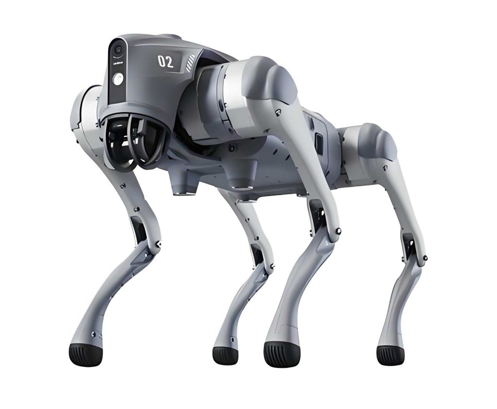
The stability and agility of legged locomotion, particularly in quadrupeds, present a fascinating and complex challenge in robotics. For a bionic robot dog tasked with navigating potentially uneven terrain in, for instance, power facility inspection, efficient and stable gait planning is paramount. Traditional approaches to gait generation often rely on meticulously crafted mathematical models of the robot’s dynamics. While effective, these methods can be brittle, requiring precise parameter tuning and struggling to generalize or adapt to unforeseen disturbances. This work explores an alternative paradigm: employing Deep Reinforcement Learning (DRL) to automatically discover effective locomotion policies. Specifically, I focus on the application of the Deep Q-Network (DQN) algorithm to plan and control the gait of a simulated bionic robot dog, with the goal of achieving fast, stable, and continuous walking without explicit dynamic modeling.
The core problem can be framed within the reinforcement learning (RL) paradigm. An agent, in this case the controller for the robot dog, learns to interact with an environment (the physics simulation). At each discrete timestep $$t$$, the agent observes a state $$s_t$$ from the environment, executes an action $$a_t$$, and receives a scalar reward $$r_t$$ and a new state $$s_{t+1}$$. The objective is to learn a policy $$\pi$$ that maps states to actions to maximize the expected cumulative future reward, or return. This return is often a discounted sum:
$$G_t = r_t + \gamma r_{t+1} + \gamma^2 r_{t+2} + … = \sum_{k=0}^{\infty} \gamma^k r_{t+k}$$
where $$\gamma \in [0, 1]$$ is the discount factor, weighting the importance of immediate versus future rewards. The optimal policy $$\pi^*$$ is the one that maximizes the state-value function $$V^{\pi}(s) = \mathbb{E}_{\pi}[G_t | s_t = s]$$ for all states. A closely related concept is the action-value function $$Q^{\pi}(s, a)$$, which defines the expected return starting from state $$s$$, taking action $$a$$, and thereafter following policy $$\pi$$:
$$Q^{\pi}(s, a) = \mathbb{E}_{\pi}[G_t | s_t = s, a_t = a]$$
The optimal Q-function satisfies the Bellman optimality equation:
$$Q^{*}(s, a) = \mathbb{E}[r + \gamma \max_{a’} Q^{*}(s’, a’) | s, a]$$
where $$s’$$ is the next state. Q-Learning is a model-free RL algorithm that directly approximates $$Q^{*}(s, a)$$ by iteratively updating estimates using the temporal difference error:
$$Q(s_t, a_t) \leftarrow Q(s_t, a_t) + \alpha [ r_t + \gamma \max_{a} Q(s_{t+1}, a) – Q(s_t, a_t) ]$$
where $$\alpha$$ is the learning rate. However, Q-Learning requires storing a Q-table, which is infeasible for high-dimensional state spaces like those describing a robot dog’s configuration. This is where DQN comes in.
The Deep Q-Network (DQN) algorithm combines Q-Learning with deep neural networks. Instead of a table, a neural network parameterized by weights $$\theta$$ is used as a function approximator for the Q-value: $$Q(s, a; \theta) \approx Q^{*}(s, a)$$. The network takes the state as input and outputs Q-values for each possible action. Two key innovations stabilize training: a target network and experience replay. The target network, with parameters $$\theta^-$$, is a periodically updated copy of the main online network. Experience replay stores transition tuples $$(s_t, a_t, r_t, s_{t+1})$$ in a buffer, and training batches are sampled randomly from this buffer to break temporal correlations. The loss function for updating the online network is the mean-squared error between the current Q-value and the target Q-value:
$$\mathcal{L}(\theta) = \mathbb{E}_{(s,a,r,s’) \sim \mathcal{D}} \left[ \left( r + \gamma \max_{a’} Q(s’, a’; \theta^-) – Q(s, a; \theta) \right)^2 \right]$$
where $$\mathcal{D}$$ is the replay buffer. This formulation allows the DQN to learn from rich sensory input and manage complex, high-dimensional control tasks like gait generation for a robot dog.
| Component | Traditional Model-Based Approach | DQN-Based Approach |
|---|---|---|
| Core Requirement | Accurate dynamics/kinematics model. | Defined state/action space and reward function. |
| Adaptability | Low; requires re-tuning for new conditions. | High; can adapt through continued learning. |
| Generalization | Limited to modeled scenarios. | Potentially generalizes across similar tasks. |
| Development Complexity | High (mathematical modeling). | High (reward engineering, training). |
The architecture for controlling the bionic robot dog based on DQN involves three main modules: Perception, Decision, and Execution. For this simulation study, the Perception module provides proprioceptive state data (joint angles, body orientation). The Decision module is where the trained DQN controller resides. The Execution module carries out the low-level motor commands. The critical design steps are in the Decision module: defining the state and action spaces for the robot dog, crafting a suitable reward function, and implementing the DQN training loop.
To apply DQN, the problem must be formulated as a Markov Decision Process (MDP). The state space $$S$$ must contain sufficient information for the robot dog to make a decision. I define the state as a 24-dimensional vector concatenating the current and previous 12-dimensional action vectors. This provides the policy with a sense of temporal continuity and recent movement history.
$$S_t = [a_t, a_{t-1}]^T \quad \text{(dimension: 24)}$$
The action space $$A$$ defines what the robot dog can do. The simulated robot dog has 12 degrees of freedom (3 joints per leg: hip, knee, ankle). The action is defined as the vector of target angular positions for all 12 joints:
$$A = q^T = [q_{n1}, q_{n2}, q_{n3}, q_{n4}, q_{m1}, q_{m2}, q_{m3}, q_{m4}, q_{k1}, q_{k2}, q_{k3}, q_{k4}]^T \quad \text{(dimension: 12)}$$
| State Space Component | Description | Dimension |
|---|---|---|
| Current Action Vector ($$a_t$$) | Target angles for all 12 joints at time $$t$$. | 12 |
| Previous Action Vector ($$a_{t-1}$$) | Target angles for all 12 joints at time $$t-1$$. | 12 |
| Total State Dimension | 24 |
The reward function is the most crucial element for guiding the learning process. It must encapsulate the desired behavior: moving forward quickly while maintaining stability. I design a composite reward function with three key components: forward progress, body stability (roll and pitch), and step regularity.
$$r_{total} = k_1 \cdot r_{forward} + k_2 \cdot (r_{roll} + r_{pitch}) + k_3 \cdot r_{step}$$
$$r_{forward} = 3 \cdot \Delta x$$
Where $$\Delta x$$ is the forward displacement of the robot dog’s torso along the global x-axis.
$$
r_{roll} =
\begin{cases}
(0.05 – |\Delta \theta_{roll}|) \times 20, & \text{if } |\Delta \theta_{roll}| \le 0.05 \text{ rad}\\
-1, & \text{otherwise}
\end{cases}
$$
$$
r_{pitch} =
\begin{cases}
(0.05 – |\Delta \theta_{pitch}|) \times 20, & \text{if } |\Delta \theta_{pitch}| \le 0.05 \text{ rad}\\
-1, & \text{otherwise}
\end{cases}
$$
Where $$\Delta \theta_{roll}$$ and $$\Delta \theta_{pitch}$$ are the changes in the robot dog’s body roll and pitch angles between steps. This penalizes large tilts, encouraging a stable torso.
$$
r_{step} =
\begin{cases}
\Delta q \times 6, & \text{if } 0.08 \text{ m} \le \Delta q \le 0.15 \text{ m}\\
-1, & \text{if } \Delta q < 0.08 \text{ m or } \Delta q > 0.15 \text{ m}
\end{cases}
$$
Where $$\Delta q$$ is the stride length. This encourages the robot dog to take reasonable, consistent steps, preventing mincing or over-extended gaits.
| Reward Component | Symbol | Purpose | Weight ($$k_i$$) |
|---|---|---|---|
| Forward Progress | $$r_{forward}$$ | Maximize forward speed. | 0.4 |
| Roll Stability | $$r_{roll}$$ | Minimize side-to-side tilt. | 0.2 |
| Pitch Stability | $$r_{pitch}$$ | Minimize front-to-back tilt. | 0.2 |
| Step Regularity | $$r_{step}$$ | Encourage optimal stride length. | 0.1 |
The DQN controller is trained in the Webots robotic simulation environment. A model of a quadrupedal robot dog with 12 actuated joints is created. The DQN network architecture consists of an input layer (24 neurons), two hidden layers (128 neurons each with ReLU activation), and an output layer (12 neurons, one for each joint’s Q-value). The training process uses an $$\epsilon$$-greedy policy for exploration, where $$\epsilon$$ decays from 0.9 to 0.1 over the training episodes to transition from exploration to exploitation. Key hyperparameters are detailed below.
| Hyperparameter | Symbol/Name | Value |
|---|---|---|
| Learning Rate | $$\alpha$$ | 0.01 |
| Discount Factor | $$\gamma$$ | 0.9 |
| Replay Buffer Size | $$\mathcal{D}$$ | 2000 |
| Batch Size | $$N$$ | 32 |
| Target Network Update Frequency | $$C$$ | Every 30 episodes |
| Initial Exploration Rate | $$\epsilon_{start}$$ | 0.9 |
| Final Exploration Rate | $$\epsilon_{end}$$ | 0.1 |
| Number of Training Episodes | $$E$$ | 400 |
The robot dog is trained for 400 episodes on flat ground. Each episode terminates after a fixed duration or if the robot dog falls. The training metrics reveal the learning progression. The loss function, which measures the error between the predicted and target Q-values, shows a clear trend of convergence. Initially high due to random predictions, the loss decreases sharply as the network begins to learn viable policies and stabilizes after approximately 80 episodes, indicating that the Q-value estimates are becoming consistent and accurate for the bionic robot dog.
$$ \mathcal{L}_{epoch} = \frac{1}{N} \sum_{i=1}^{N} (y_i – Q(s_i, a_i; \theta))^2 $$
The learned gait’s performance is evaluated by analyzing the robot dog’s motion data. The forward displacement over time shows a near-linear progression, confirming that the robot dog achieves a steady walking pace. The torso height remains stable around 0.7 meters, demonstrating successful posture control. An analysis of the foot trajectory for a single leg shows a cyclical pattern with a stride length of approximately 0.3 meters (swing in x-direction from -0.15m to 0.15m) and a foot clearance of about 0.05 meters (swing in z-direction), forming a biologically plausible swing-stance cycle.
Most importantly, the body orientation angles—roll and pitch—oscillate within a very small band around zero. While minor fluctuations are present due to the discrete nature of the control actions, the overall trend is stable. This directly fulfills the objective encoded in the reward function and proves the DQN controller’s effectiveness in maintaining the robot dog’s balance during locomotion. The successful stabilization of these angles is a strong indicator of a viable, stable gait for the simulated robot dog.
The evolution of the reward components provides further insight. The average total reward per episode increases significantly during the first 100 episodes and then plateaus at a high value, signifying that the policy has converged to a near-optimal one. The individual reward components for forward progress, roll stability, and pitch stability all show a similar rising-and-plateauing trend, confirming that the robot dog is simultaneously improving in all desired aspects. The step regularity reward also stabilizes, indicating the emergence of a consistent walking rhythm. This comprehensive improvement across all reward metrics validates the design of the composite reward function for training the bionic robot dog.
In conclusion, this work demonstrates a successful application of the DQN reinforcement learning algorithm for gait planning in a bionic robot dog. By framing locomotion as an RL problem with a carefully designed state space, action space, and multi-component reward function, a neural network controller was trained to produce stable, continuous, and effective walking without requiring an explicit analytical model of the robot’s dynamics. The controller, trained entirely in simulation, learned to coordinate 12 joints to maximize forward speed while minimizing body tilt and maintaining regular strides. The convergence of the loss function and the stabilization of key performance metrics (roll, pitch, forward speed) provide empirical evidence of the method’s efficacy. This model-free, learning-based approach offers a promising and flexible alternative to traditional model-based control for legged robots like the robot dog, particularly for adapting to complex terrains where analytical models become intractable. Future work will involve transferring the policy to physical hardware, training on varied and uneven terrain, and exploring more advanced DRL algorithms like DDPG or PPO for continuous action spaces to achieve even smoother and more dynamic motions for the versatile robot dog.