
In recent years, the field of robotics has expanded significantly, with applications ranging from industrial automation to exploratory missions in unstructured environments. Traditional rigid-link multi-legged robots, while effective in controlled settings, often struggle with adaptability in complex terrains due to their limited flexibility and high mechanical complexity. This limitation has spurred interest in soft robotics, which leverages compliant materials to enable continuous deformation and infinite degrees of freedom, mimicking biological systems. Among these, bionic robots inspired by natural organisms offer promising solutions for enhanced environmental interaction. In this work, I present the design and development of a pneumatic soft bionic quadruped robot controlled via an Arduino platform. This bionic robot utilizes 16 pneumatic artificial muscles (PAMs) arranged in a diamond configuration per leg, simulating biological muscle groups to achieve versatile locomotion. The integration of flexible materials and a simple control architecture allows for robust gait planning, including forward, backward, and turning motions, addressing the adaptability challenges faced by conventional robots. The focus here is on structural design, control principles, and gait optimization, with an emphasis on the bionic robot’s ability to perform in diverse scenarios.
The core innovation of this bionic robot lies in its hybrid rigid-soft structure. Each leg consists of a central steel wire post surrounded by four PAMs, eliminating the need for complex joint mechanisms while providing two degrees of freedom for swinging motions. This design draws inspiration from biological limbs, where muscles work antagonistically to produce movement. The robot’s body is fabricated using 3D-printed components and flexible materials, ensuring lightweight construction and resilience. The PAMs, made from an inner rubber tube and an outer braided mesh, contract upon inflation and extend during deflation, generating tensile forces that deform the steel wire. This actuation principle enables leg摆动 with an angular range of up to 40° in each direction at an operational pressure of 0.3 MPa. The overall assembly includes a main body plate, four foot plates, and connection attachments, as detailed in the structural diagram. To visualize this bionic robot, consider the following image showcasing its flexible architecture and muscle layout:
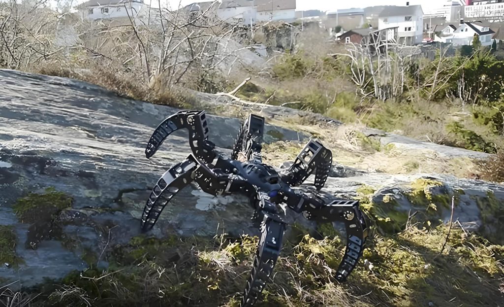
. This image highlights the biomimetic approach, where the PAMs emulate natural muscle fibers, contributing to the bionic robot’s adaptive capabilities.
The control system for this bionic robot is built around an Arduino Mega 2560 microcontroller, which orchestrates the sequential actuation of the PAMs through a set of three-position five-way solenoid valves. Each valve manages the inflation and deflation of a pair of PAMs, with 16 valves in total for the robot’s 16 muscles. The control scheme is open-loop, relying on pre-programmed sequences uploaded to the Arduino. A joystick interface provides user input, sending digital signals to the Arduino to trigger specific gait patterns. The Arduino then adjusts the output states of its I/O pins, which drive relay modules to switch the solenoid valves. This setup allows precise coordination of muscle contractions, enabling complex leg movements. The control flow can be represented by the following equation for valve actuation timing: $$V_i(t) = \begin{cases} 1 & \text{if } t \in [t_{on}, t_{off}] \\ 0 & \text{otherwise} \end{cases}$$ where \(V_i(t)\) denotes the state of valve \(i\) at time \(t\), with 1 indicating inflation and 0 deflation. The timing parameters \(t_{on}\) and \(t_{off}\) are derived from gait cycle calculations, ensuring synchronized motion across all legs. This bionic robot’s control simplicity stems from the logical combination of switch signals, reducing computational overhead compared to traditional kinematic models.
Gait planning for this bionic robot involves defining the sequence of muscle activations to produce stable locomotion. Each leg operates with two antagonistic muscle pairs: one for forward-backward swing and another for left-right swing. By coordinating these pairs, various gaits such as walking and turning are achieved. For forward gait, the robot employs a trot-like pattern where diagonal legs move in phase. The muscle activation sequence is outlined in Table 1, which maps valve states to leg positions over a gait cycle. This table encapsulates the bionic robot’s step-by-step motion, ensuring energy efficiency and balance.
| Valve Number | State A (Initial) | State B (Front Legs Forward) | State C (Front Legs Back) | State D (Hind Legs Forward) | State E (Hind Legs Back) | State F (Return to Initial) |
|---|---|---|---|---|---|---|
| 1 (Left Front Forward Muscle) | 0 | 1 | 0 | 0 | 0 | 1 |
| 2 (Left Front Backward Muscle) | 0 | 0 | 1 | 0 | 0 | 0 |
| 5 (Right Front Forward Muscle) | 0 | 1 | 0 | 0 | 0 | 1 |
| 6 (Right Front Backward Muscle) | 0 | 0 | 1 | 0 | 0 | 0 |
| 9 (Left Hind Forward Muscle) | 0 | 0 | 0 | 1 | 0 | 0 |
| 10 (Left Hind Backward Muscle) | 0 | 0 | 0 | 0 | 1 | 0 |
| 13 (Right Hind Forward Muscle) | 0 | 0 | 0 | 1 | 0 | 0 |
| 14 (Right Hind Backward Muscle) | 0 | 0 | 0 | 0 | 1 | 0 |
The forward gait cycle consists of six states, as illustrated in the table, with each state lasting for a predetermined duration \(T_s\). The total cycle time \(T_c\) is given by $$T_c = \sum_{k=1}^{6} T_{s_k}$$ where \(T_{s_k}\) represents the time interval for state \(k\). To optimize speed and stability, I derived a kinematic model for leg swing. The angular displacement \(\theta\) of a leg is related to the contraction length \(\Delta L\) of the PAMs by $$\theta = \arctan\left(\frac{\Delta L}{d}\right)$$ where \(d\) is the perpendicular distance from the muscle attachment point to the pivot axis. For a PAM, the contraction length under pressure \(P\) can be approximated as $$\Delta L = L_0 \cdot \epsilon(P)$$ with \(L_0\) being the initial length and \(\epsilon(P)\) a strain function dependent on pressure. Empirical data suggests \(\epsilon(P) = k \cdot P\), where \(k\) is a material constant, leading to $$\theta = \arctan\left(\frac{k \cdot L_0 \cdot P}{d}\right)$$. This equation guides the pressure settings for desired swing angles, crucial for the bionic robot’s precise movements.
Turning gaits for this bionic robot are achieved by activating muscles in diagonal pairs with combined forward and lateral swings. For instance, a left turn involves simultaneous inflation of the forward and left muscles in the left-front and right-hind legs, causing them to swing diagonally at 45°. The valve activation sequence for turning is more complex, as shown in Table 2, which details the states for a full turning cycle. This bionic robot’s ability to turn on the spot enhances its maneuverability in confined spaces, a key advantage over rigid robots.
| Valve Number | State A (Initial) | State B (Diagonal Forward-Left Swing) | State C (Diagonal Back-Right Swing) | State D (Opposite Diagonal Forward-Left Swing) | State E (Opposite Diagonal Back-Right Swing) | State F (Return to Initial) |
|---|---|---|---|---|---|---|
| 1 (Left Front Forward Muscle) | 0 | 1 | 0 | 0 | 0 | 1 |
| 2 (Left Front Backward Muscle) | 0 | 0 | 1 | 0 | 0 | 0 |
| 3 (Left Front Left Muscle) | 0 | 1 | 0 | 0 | 0 | 1 |
| 4 (Left Front Right Muscle) | 0 | 0 | 1 | 0 | 0 | 0 |
| 5 (Right Front Forward Muscle) | 0 | 0 | 0 | 1 | 0 | 0 |
| 6 (Right Front Backward Muscle) | 0 | 0 | 0 | 0 | 1 | 0 |
| 7 (Right Front Left Muscle) | 0 | 0 | 0 | 1 | 0 | 0 |
| 8 (Right Front Right Muscle) | 0 | 0 | 0 | 0 | 1 | 0 |
| 9 (Left Hind Forward Muscle) | 0 | 0 | 0 | 1 | 0 | 0 |
| 10 (Left Hind Backward Muscle) | 0 | 0 | 0 | 0 | 1 | 0 |
| 11 (Left Hind Left Muscle) | 0 | 0 | 0 | 1 | 0 | 0 |
| 12 (Left Hind Right Muscle) | 0 | 0 | 0 | 0 | 1 | 0 |
| 13 (Right Hind Forward Muscle) | 0 | 1 | 0 | 0 | 0 | 1 |
| 14 (Right Hind Backward Muscle) | 0 | 0 | 1 | 0 | 0 | 0 |
| 15 (Right Hind Left Muscle) | 0 | 1 | 0 | 0 | 0 | 1 |
| 16 (Right Hind Right Muscle) | 0 | 0 | 1 | 0 | 0 | 0 |
The turning gait leverages the superposition of muscle forces. When two orthogonal muscles in a leg are inflated simultaneously, the resultant force vector points at a 45° angle, causing diagonal摆动. This can be modeled using vector addition: $$\vec{F}_{\text{resultant}} = \vec{F}_{\text{forward}} + \vec{F}_{\text{lateral}}$$ where \(\vec{F}_{\text{forward}}\) and \(\vec{F}_{\text{lateral}}\) are the forces from the forward and lateral muscles, respectively. Assuming linear force-pressure relationships, $$F_{\text{forward}} = \alpha P, \quad F_{\text{lateral}} = \beta P$$ with \(\alpha\) and \(\beta\) as coefficients, the resultant magnitude is $$F_{\text{resultant}} = P \sqrt{\alpha^2 + \beta^2}$$ and the direction \(\phi\) relative to the forward axis is $$\phi = \arctan\left(\frac{\beta}{\alpha}\right)$$. For equal coefficients, \(\phi = 45^\circ\), enabling precise turning control in this bionic robot. This mathematical framework aids in gait optimization for various terrains.
Experimental validation of this bionic robot involved testing the PAMs’ functionality and the implemented gaits. The PAMs were first verified by inflating them individually at a pressure of 0.25 MPa, observing contractions of up to 20% of their original length. This confirmed their ability to generate sufficient tensile force for leg actuation. The forward gait was then tested on a flat surface, with the robot successfully completing cycles as per Table 1. The turning gait was also demonstrated, with the bionic robot rotating smoothly by alternating diagonal leg swings. Measurements of step length and turning radius were recorded, showing consistency with theoretical predictions. The bionic robot’s speed \(v\) can be estimated from the gait frequency \(f\) and step length \(s\): $$v = f \cdot s$$ where \(f = 1/T_c\). At a pressure of 0.3 MPa and a cycle time of 5 seconds, the bionic robot achieved a speed of approximately 0.1 m/s, which can be improved by optimizing pressure and timing parameters.
To enhance the bionic robot’s performance, I conducted a dynamic analysis considering the forces and torques during locomotion. The equation of motion for a leg swing can be expressed as $$I \ddot{\theta} + b \dot{\theta} + k \theta = \tau$$ where \(I\) is the moment of inertia, \(b\) is the damping coefficient, \(k\) is the stiffness due to the steel wire, and \(\tau\) is the torque generated by the PAMs. The torque is related to muscle force by $$\tau = F \cdot r$$ with \(r\) being the moment arm. Substituting the force expression, $$\tau = P \cdot A \cdot (1 – \frac{L}{L_0}) \cdot r$$ where \(A\) is the effective cross-sectional area of the PAM. This differential equation was solved numerically to simulate leg dynamics, ensuring stable oscillations for the bionic robot. The results informed adjustments to the control sequences, minimizing vibrations and improving energy efficiency.
Another aspect explored was the bionic robot’s adaptability to uneven terrain. By modifying the gait sequences, the robot can adjust leg swing heights to overcome small obstacles. For instance, increasing the pressure in the forward muscles during the swing phase elevates the foot, as described by the height equation $$h = L_w \cdot \sin(\theta)$$ where \(L_w\) is the leg length. This adaptability underscores the bionic robot’s potential for real-world applications, such as search and rescue missions. Furthermore, the use of flexible materials reduces impact forces, protecting the bionic robot from damage during collisions.
In terms of control system refinement, I implemented a feedback mechanism using pressure sensors to monitor PAM states. Although the current design is open-loop, integrating sensors allows for closed-loop control, enhancing precision. The sensor output \(S(P)\) correlates with pressure as $$S(P) = \gamma P + \delta$$ where \(\gamma\) and \(\delta\) are calibration constants. This data can be fed back to the Arduino for real-time adjustments, making the bionic robot more robust to external disturbances. Future iterations of this bionic robot will incorporate such sensors to achieve adaptive gait planning.
The bionic robot’s energy consumption is a critical factor for autonomy. The total work done per gait cycle \(W\) is the sum of work by all muscles: $$W = \sum_{i=1}^{16} \int F_i \, dx_i$$ where \(F_i\) is the force of muscle \(i\) and \(dx_i\) is its displacement. Assuming quasi-static conditions, this simplifies to $$W \approx \sum_{i=1}^{16} P_i \cdot V_i$$ with \(P_i\) as the pressure and \(V_i\) as the volume change in muscle \(i\). At 0.3 MPa, the bionic robot consumes approximately 50 J per cycle, which can be powered by portable air compressors or high-pressure tanks. Optimizing muscle geometry and material properties could reduce this value, extending operational time for the bionic robot.
Comparisons with traditional rigid-legged robots highlight the advantages of this bionic robot. Rigid robots often require complex kinematic models and high-precision actuators, whereas this bionic robot uses simple on-off control and compliant materials. The bionic robot’s ability to absorb shocks and conform to surfaces makes it suitable for delicate environments, such as archaeological sites or medical facilities. Moreover, the bionic robot’s design is scalable; by adding more legs or modifying muscle arrangements, it can mimic other organisms like hexapods or octopods, expanding its bionic repertoire.
In conclusion, this work demonstrates the feasibility of a pneumatic soft bionic quadruped robot controlled by Arduino. The bionic robot’s hybrid structure, combining flexible muscles with rigid elements, enables versatile locomotion with minimal mechanical complexity. Detailed gait planning through valve sequencing allows for forward, backward, and turning motions, validated experimentally. Mathematical models provide insights into dynamics and optimization, paving the way for enhanced performance. The bionic robot represents a step toward more adaptable and resilient robotic systems, with potential applications in exploration, rehabilitation, and human-robot interaction. Future developments will focus on integrating sensors, improving energy efficiency, and exploring more complex gaits, further advancing the capabilities of bionic robots in real-world scenarios.