
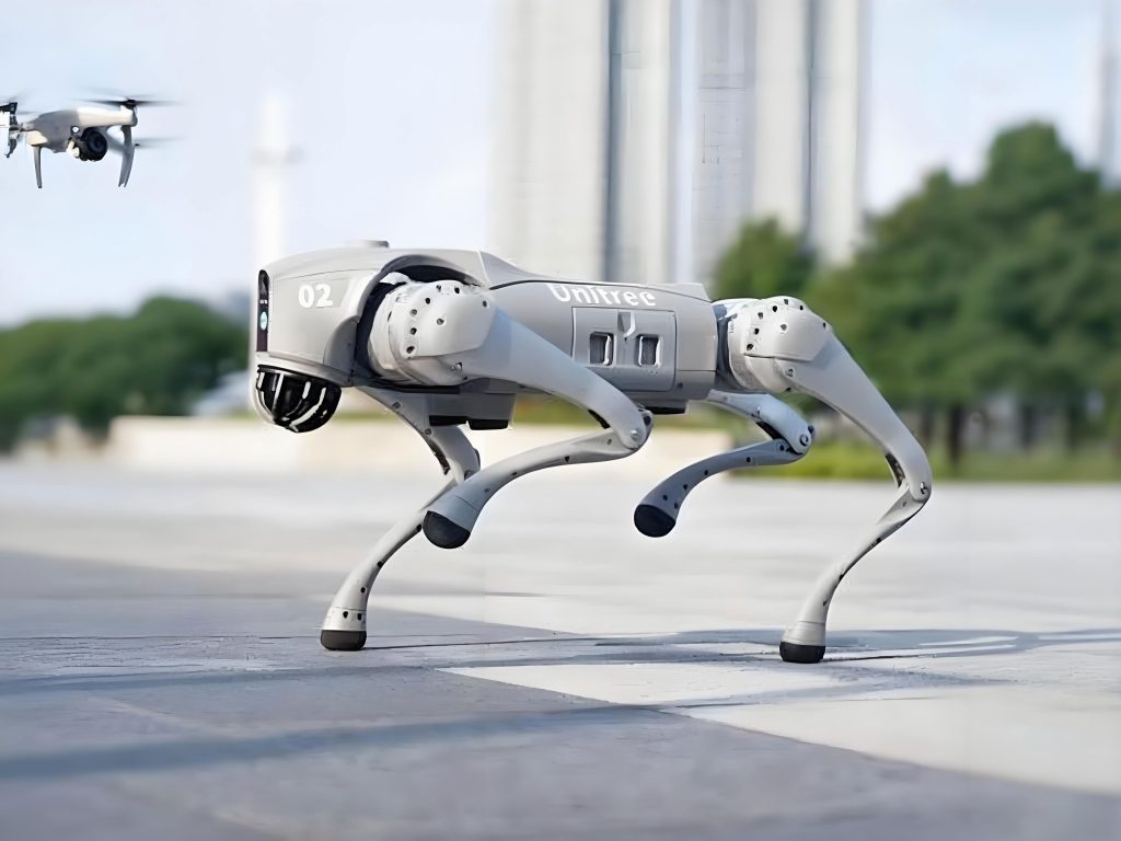
The development of legged locomotion systems represents a significant frontier in robotics, offering the potential for unprecedented mobility in complex, unstructured environments. Among these, the quadruped bionic robot stands out due to its inherent stability, dynamic capability, and high load-bearing potential, drawing direct inspiration from biological quadrupeds in nature. The research and realization of such sophisticated machines involve immense challenges in mechanical design, control architecture, and algorithmic development. In this context, dynamics simulation emerges as an indispensable tool. It provides a virtual proving ground that is both cost-effective and risk-free, enabling researchers to iterate on designs, develop and debug control algorithms, and predict system behavior under a vast array of conditions long before physical prototypes are built. This report details the methodology and implementation of a dynamics simulation framework for a quadruped bionic robot, specifically focusing on a force-control paradigm, which is crucial for achieving dynamic, robust, and energy-efficient locomotion.
The core of any realistic simulation lies in an accurate and computationally tractable model. Our quadruped bionic robot model is inspired by mammalian morphology, featuring a torso and four articulated limbs. Each leg is kinematically modeled as a serial chain with four degrees of freedom (DoF): a hip abduction/adduction joint, a hip flexion/extension joint, a knee flexion/extension joint, and an ankle flexion/extension joint. This configuration provides substantial dexterity for omnidirectional movement and posture adjustment. For clarity in control and analysis, we adopt a standard nomenclature for the legs: Left Front (LF), Right Front (RF), Left Hind (LH), and Right Hind (RH). Each joint angle is denoted as $q_i$, where $i = 1, 2, …, 16$, sequentially covering all joints from LF to RH.
The geometric and inertial properties of each link are fundamental to dynamic calculations. We define a comprehensive set of parameters for every link in the robot’s kinematic tree. These parameters are essential for both kinematic computations and the dynamic algorithms that will be employed. The table below summarizes the key parameters used in our simulation model.
| Symbol | Description |
|---|---|
| $q$ | Joint angle (scalar for revolute joints) |
| $\dot{q}$ | Joint angular velocity |
| $\ddot{q}$ | Joint angular acceleration |
| $\mathbf{a}$ | Joint axis unit vector (expressed in parent link frame) |
| $\mathbf{b}$ | Position vector from parent link frame to this joint frame |
| $\mathbf{p}$ | Position of the joint in the world coordinate frame |
| $\mathbf{R}$ | Orientation matrix of the joint/link in the world frame |
| $\mathbf{v}$ | Linear velocity of the link origin in the world frame |
| $\boldsymbol{\omega}$ | Angular velocity of the link in the world frame |
| $m$ | Mass of the link |
| $\mathbf{c}$ | Position of the link’s center of mass (CoM) in the world frame |
| $\mathbf{I}$ | Inertia tensor of the link about its CoM, expressed in the world frame |
Kinematic Foundation
Accurate motion planning and control for the quadruped bionic robot begin with a solid kinematic model. We employ the spatial vector algebra formalism, which provides a compact and efficient way to represent rigid body motions and forces. The forward kinematics of the robot, which computes the pose (position and orientation) of any link given the joint angles, is built recursively from the torso (base) outwards to the foot tips. For a joint $i$, the spatial velocity $\mathcal{V}_i$ (a 6D vector combining linear and angular velocity) is propagated as:
$$
\mathcal{V}_i = \mathbf{X}_i \mathcal{V}_{\text{parent}(i)} + \mathbf{s}_i \dot{q}_i
$$
where $\mathbf{X}_i$ is the spatial transformation from the parent link frame to the current link frame, $\mathcal{V}_{\text{parent}(i)}$ is the spatial velocity of the parent link, and $\mathbf{s}_i$ is the joint motion subspace vector (e.g., $(0,0,0,0,0,1)^T$ for a rotational joint about the local z-axis). The acceleration propagation includes the Coriolis and centrifugal terms:
$$
\dot{\mathcal{V}}_i = \mathbf{X}_i \dot{\mathcal{V}}_{\text{parent}(i)} + \mathbf{s}_i \ddot{q}_i + \dot{\mathbf{X}}_i \mathcal{V}_{\text{parent}(i)} + \mathbf{s}_i \dot{q}_i \times \mathcal{V}_i
$$
Here, the operator $\times$ denotes the spatial cross product. The inverse kinematics, critical for determining joint angles from desired foot placements, is solved numerically for this complex, redundant limb structure, often using Jacobian-based methods like the pseudo-inverse to handle the null-space motion for posture optimization.
Dynamic Modeling and the Force Control Paradigm
Simulating the realistic motion of a bionic robot necessitates solving its dynamics. There are two fundamental problems: forward dynamics (calculating acceleration from forces) and inverse dynamics (calculating forces from a known motion). For motion control, especially in a force-control mode, inverse dynamics is paramount. It allows us to compute the precise joint torques required to produce a desired body and limb trajectory, accounting for all inertial, Coriolis, centrifugal, and gravitational effects.
We implement the Recursive Newton-Euler Algorithm (RNEA), an O(n) algorithm renowned for its computational efficiency, to solve the inverse dynamics problem for our quadruped bionic robot. The algorithm operates in two sweeps across the kinematic tree: an outward sweep to compute velocities and accelerations, and an inward sweep to compute forces and torques.
Outward Sweep: Velocity and Acceleration Propagation
Starting from the known state of the torso (which may have free-floating base dynamics or be fixed for simpler models), we propagate motion to the leaves (feet). For each link $i$, connected to its parent by joint $i$, we compute its spatial velocity $\mathcal{V}_i$ and acceleration $\dot{\mathcal{V}}_i$ as shown in the kinematic equations above. The initial conditions for the torso’s spatial acceleration include the gravitational acceleration: $\dot{\mathcal{V}}_0 = (-\mathbf{g}, \mathbf{0})$.
Inward Sweep: Force and Torque Computation
After the outward sweep, we know the motion of every link. The inward sweep calculates the forces required to produce this motion. For a link $i$, the net spatial force $\mathcal{F}_i$ acting on it is given by the Newton-Euler equation in spatial form:
$$
\mathcal{F}_i = \mathbf{I}_i \dot{\mathcal{V}}_i + \mathcal{V}_i \times^* \mathbf{I}_i \mathcal{V}_i
$$
Here, $\mathbf{I}_i$ is the spatial inertia matrix of link $i$, and $\times^*$ is the spatial cross-product dual operator. This net force has contributions from the parent link force $\mathcal{F}_{\lambda(i)}$, the force from any child link $\mathcal{F}_{C(i)}$, and external forces $\mathcal{F}^e_i$ (like ground reaction forces at the foot). The force exerted by the parent link onto link $i$ is therefore:
$$
\mathcal{F}^a_i = \mathcal{F}_i – \mathcal{F}^e_i – \sum_{j \in C(i)} \mathbf{X}_j^T \mathcal{F}^a_j
$$
where $\mathbf{X}_j^T$ transforms the force from child link $j$’s frame back to link $i$’s frame. Finally, the scalar joint torque $u_i$ required at joint $i$ is found by projecting this spatial force onto the joint axis:
$$
u_i = \mathbf{s}_i^T \mathcal{F}^a_i
$$
The RNEA elegantly bundles these steps. The key equations for the inward recursion, incorporating external forces $\mathcal{F}^e_i$ which are crucial for a legged bionic robot interacting with the ground, are summarized below for a link with a single child (generalizable to branching structures like a torso with four legs):
$$
\begin{aligned}
& \mathbf{f}_i = \mathbf{I}_{C,i} \dot{\mathcal{V}}_i + \mathcal{V}_i \times^* \mathbf{I}_{C,i} \mathcal{V}_i – \mathbf{X}_j^T \mathbf{f}_j – \mathcal{F}^e_i \\
& u_i = \mathbf{s}_i^T \mathbf{f}_i
\end{aligned}
$$
Here, $\mathbf{I}_{C,i}$ is the composite spatial inertia of the subtree rooted at link $i$, and $\mathbf{f}_i$ is the articulated-body force. This algorithm provides the exact joint torques needed to realize a prescribed motion trajectory $\mathbf{q}(t), \dot{\mathbf{q}}(t), \ddot{\mathbf{q}}(t)$, under the influence of gravity and specified external contact forces. This is the essence of force control for simulation: we command torques, not directly positions.
Architecture of the Dynamics Simulation System
To create a flexible, reusable, and modular simulation environment for the quadruped bionic robot, we architected the system based on the component-oriented principles of a Robot Technology Middleware (RTM). This approach decouples functionalities into independent, communicating components, facilitating development, testing, and integration of new algorithms. The system comprises several key components, as illustrated in the following workflow description.
| Module | Primary Function |
|---|---|
| Model Loader & Visualizer | Loads the geometric (e.g., VRML) and dynamic (mass, inertia) models of the robot and environment into the 3D simulation scene. It sends parameters to the dynamics engine and geometry data to the collision detector. |
| Virtual Sensor Model | Emulates sensors like joint encoders, inertial measurement units (IMUs), foot force sensors, and depth cameras. It queries the simulation state to generate realistic sensor data for the controller. |
| Motion Controller | The brain of the operation. It ingests virtual sensor data, runs high-level gait algorithms (e.g., trot, pace, walk) and balance controllers, and outputs either desired joint positions/velocities or, in our case, desired joint torques. This module houses the RNEA for inverse dynamics computation. |
| Dynamics Engine | The physics core. It integrates the equations of motion. In the force-control mode, it applies the torques computed by the Motion Controller, along with gravity and contact forces, to compute new joint accelerations. It then performs numerical integration (e.g., Runge-Kutta) to update joint velocities and positions. |
| Collision Detection | Continuously checks for intersections between robot geometry and the environment. It provides information such as contact points, normals, and penetration depths to the Dynamics Engine, which then resolves these collisions using a contact model (e.g., spring-damper, penalty method, or complementarity-based). |
| System Supervisor | Orchestrates data flow between components, manages simulation timing (real-time or faster), and provides user interfaces for starting, stopping, and monitoring simulations. |
The data flow is cyclical:
1. The Model Loader initializes the scene.
2. The Virtual Sensor Model reads the current state from the Dynamics Engine.
3. The Motion Controller processes sensor data, plans the motion, and uses RNEA to compute required joint torques $\mathbf{u}$.
4. These torques $\mathbf{u}$ and any external contact forces $\mathcal{F}^e$ (from collision response) are sent to the Dynamics Engine.
5. The Dynamics Engine computes the new state (accelerations, then velocities, then positions) for the next time step.
6. The Collision Detection module updates contact information based on the new state.
7. The Visualizer renders the new state.
8. The loop repeats from step 2.
This modular architecture is particularly advantageous for a bionic robot platform, as it allows for easy swapping of control algorithms, contact models, or even entire robot models without overhauling the entire system.
Simulation Experiment: Trotting Gait
To validate our force-control-based simulation framework, we conducted an experiment commanding the quadruped bionic robot to perform a trotting gait. The trot is a dynamic, diagonal-synchronized gait where the LF and RH legs move in phase, and the RF and LH legs move in the opposite phase. It offers a good balance of speed and stability, making it a standard test for legged robot locomotion.
Gait Planning: We defined a periodic gait cycle with a frequency of 1.5 Hz. The foot trajectory for each swing leg was prescribed as an elliptical path in Cartesian space relative to the hip, ensuring ground clearance and smooth touch-down/lift-off. The stance legs were commanded to provide support and propel the body forward. The desired joint angles $\mathbf{q}^d(t)$, velocities $\dot{\mathbf{q}}^d(t)$, and accelerations $\ddot{\mathbf{q}}^d(t)$ for all 16 joints were generated through a combination of inverse kinematics (for swing legs) and torso posture control (for stance legs).
Inverse Dynamics Computation: At each simulation time step, the Motion Controller executed the RNEA. The inputs were:
• The desired motion trajectory ($\mathbf{q}^d, \dot{\mathbf{q}}^d, \ddot{\mathbf{q}}^d$).
• The model parameters (masses, inertias, link lengths).
• The external forces $\mathcal{F}^e_i$. For swing legs, $\mathcal{F}^e_i$ was set to zero (only gravity is accounted for in the inertia terms). For stance legs, $\mathcal{F}^e_i$ represented the ground reaction force (GRF). In this simulation, the GRF was calculated using a simplified spring-damper contact model at the foot, but more advanced models like rigid-body contact with friction cones can be integrated.
The RNEA efficiently computed the required joint torque vector $\mathbf{u}(t)$ for all 16 actuators. The plots below conceptually show the resulting joint angles and torques for two key joints during several gait cycles. The torque profiles are non-linear and complex, reflecting the dynamic interactions between limbs and the torso, which a simple position controller would struggle to manage efficiently.
The joint torque $u_i$ for a leg joint during a trot cycle exhibits distinct peaks corresponding to phases of leg loading (impact, weight-bearing) and thrust generation. The equation governing this, derived from the inward recursion, is:
$$
u_i(t) = \mathbf{s}_i^T \left[ \mathbf{I}_{C,i}(\mathbf{q}) \ddot{\mathbf{q}}^d(t) + \mathbf{C}_{i}(\mathbf{q}, \dot{\mathbf{q}}) \dot{\mathbf{q}}^d(t) + \mathbf{g}_i(\mathbf{q}) – \mathbf{J}_i^T(\mathbf{q}) \mathbf{F}_{grf}(t) \right]
$$
where $\mathbf{C}_{i}$ represents Coriolis and centrifugal terms, $\mathbf{g}_i$ is the gravity term, $\mathbf{J}_i$ is the foot Jacobian, and $\mathbf{F}_{grf}$ is the ground reaction force vector at the foot. This clearly shows how the torque depends on desired acceleration, velocity-squared terms, configuration-dependent gravity, and most importantly for a force-controlled bionic robot, the external contact forces.
Simulation Execution: The computed torques $\mathbf{u}(t)$ were fed into the Dynamics Engine. The engine applied these torques, along with gravity and the simulated ground reaction forces, to numerically integrate the full equations of motion of the floating-base robot. The simulation successfully demonstrated stable, periodic trotting locomotion. The robot’s torso maintained a relatively steady height and pitch angle, while the legs cycled through their programmed trajectories. The force-control approach allowed the robot to naturally accommodate the interaction forces with the ground, resulting in a more physically plausible and stable simulation compared to pure position control, which would fight against these dynamics.
Conclusion and Future Work
This report has presented a comprehensive framework for the dynamics simulation of a quadruped bionic robot operating under force control. By leveraging an efficient recursive inverse dynamics algorithm (RNEA) within a modular, middleware-based architecture, we have created a simulation tool that accurately computes the joint torques necessary to execute complex, dynamic motions like trotting. This force-control paradigm is fundamental for developing controllers that can manage the high-dynamic interactions inherent in legged locomotion, paving the way for more robust and adaptive bionic robot systems.
The advantages of this approach are multifold: it provides high physical fidelity, enables the testing of advanced torque-based control laws (such as impedance control or whole-body control), and offers a flexible platform for algorithm development. The modular design ensures that individual components, such as the contact model, the gait planner, or the state estimator, can be improved or replaced independently.
Future work will focus on several enhancements to increase the utility and realism of the simulation for the bionic robot:
1. Advanced Contact Modeling: Integrating a rigid-body contact solver with Coulomb friction to more accurately simulate foot-ground interaction, slip, and uneven terrain.
2. Hydraulic Actuator Dynamics: Incorporating models of hydraulic actuators (common in powerful quadrupeds like BigDog), including valve dynamics, hose compliance, and piston friction, to better simulate the force-generation limitations and bandwidth.
3. Terrain Perception and Adaptation: Coupling the simulation with perception algorithms to enable the virtual bionic robot to sense and adapt its gait to complex, uneven terrain in real-time.
4. Hardware-in-the-Loop (HIL) Simulation: Connecting the simulation to actual robot hardware controllers to test and validate low-level control firmware and electronics before full deployment.
By continuing to refine this dynamics simulation platform, we accelerate the development cycle of advanced quadruped bionic robots, bringing us closer to realizing machines capable of operating alongside humans in the most challenging natural and man-made environments.