
The quest for mobile robots capable of navigating complex, unstructured terrain has driven significant research into biologically inspired locomotion. Wheeled and tracked vehicles are often limited by the terrain’s geometry and roughness. In contrast, legged animals exhibit remarkable adaptability, traversing obstacles, slopes, and irregular surfaces with ease. This inherent advantage has fueled the development of legged bionic robots, which aim to emulate the locomotion principles of creatures such as insects, spiders, and mammals. Among these, hexapod (six-legged) configurations are particularly popular due to their inherent static stability. A hexapod bionic robot can maintain balance with a simple, always-stable gait, allowing three legs to be in a swing phase while the other three provide support. This article delves deeply into the gait planning, detailed kinematic modeling, workspace analysis, and trajectory generation for a hexapod bionic robot, providing a comprehensive foundation for its control and deployment in challenging environments.
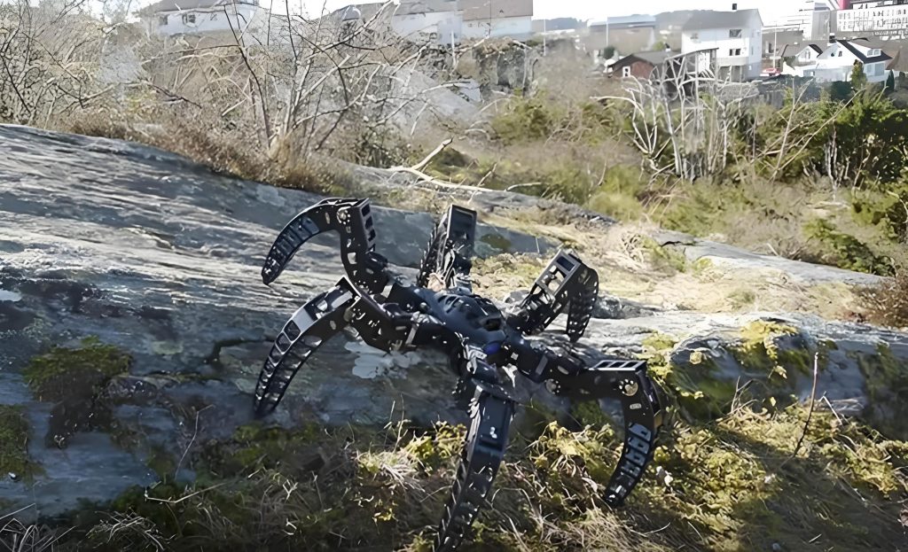
The mechanical design of a typical hexapod bionic robot is central to its functionality. The body, or chassis, serves as the central platform to which six identical legs are attached, usually in a symmetrical arrangement—three on each side. Each leg is a serial kinematic chain, most commonly featuring three rotational degrees of freedom (DOF). This configuration is inspired by insect leg morphology and provides the necessary dexterity for walking and obstacle negotiation. The three joints are typically defined as:
- Root Joint (Yaw Joint): Located where the leg connects to the body, this joint rotates about an axis perpendicular to the body plane (often the body’s vertical axis). It controls the leg’s forward/backward sweeping motion relative to the body’s heading.
- Hip Joint (Pitch Joint): This joint, adjacent to the root joint, rotates about an axis parallel to the body’s lateral axis. It primarily controls the lifting and lowering of the entire leg.
- Knee Joint (Pitch Joint): Located between the thigh and shin links, this joint also rotates about an axis parallel to the hip joint axis. It controls the extension and retraction of the lower part of the leg.
This 3-DOF design allows the foot endpoint to reach any position within a substantial volume of space beneath and around the body, which is defined as its reachable workspace.
Gait Planning for Stable Locomotion
A gait defines the sequence and timing of leg movements during locomotion. For a hexapod bionic robot, selecting an appropriate gait is crucial for stability, speed, and energy efficiency. The most fundamental and widely used gait for hexapods is the Tripod Gait. This gait leverages the robot’s six legs to create two alternating tripods of support, ensuring continuous static stability.
In the tripod gait, the six legs are divided into two mechanically interlocked groups:
- Group 1: Legs 1, 3, and 5 (typically the front and rear legs on one side and the middle leg on the opposite side).
- Group 2: Legs 2, 4, and 6 (the remaining three legs).
The gait cycle is divided into two main phases: the Stance Phase (leg on ground, propelling the body) and the Swing Phase (leg lifted, moving forward to the next foothold). In the tripod gait, when Group 1 legs are in the swing phase, Group 2 legs are in the stance phase, and vice versa. This means that at any instant, three legs (forming a stable tripod) are always in contact with the ground. The robot’s center of mass (CoM) must remain within the support polygon formed by these three foothold points to maintain static stability, a condition easily satisfied with proper body motion planning.
The timing diagram for a complete stride is as follows:
- Initial State: Group 1 legs are lifted and begin their swing phase, moving forward by half a step length. Group 2 legs are on the ground in their stance phase.
- Midpoint 1: Group 1 legs finish their swing and touch down, entering the stance phase. Simultaneously, Group 2 legs lift off to begin their swing phase.
- Body Advancement: With Group 1 now supporting the body, the entire robot body advances forward by one full step length. During this translation, the swinging legs of Group 2 move backward relative to the body, effectively preparing for their next stance.
- Midpoint 2: Group 2 legs finish their swing and touch down. Group 1 legs then lift off.
- Body Advancement: The body advances another step length while supported by Group 2.
This sequence repeats. A key simplification in this planning is the decoupling of body and leg motion: the body is stationary during leg swings, and the swinging legs are stationary relative to the body during body advancement. This simplification significantly eases the computational burden for real-time trajectory planning and control of the bionic robot.
| Gait Type | Leg Groups | Duty Factor (β) | Stability | Speed | Energy Efficiency |
|---|---|---|---|---|---|
| Tripod | 2 (3 legs each) | 0.5 | Statically Stable | High | Moderate |
| Wave | 6 (1 leg each) | > 0.5 | Very High | Low | Low |
| Tetrapod | 3 (2 legs each) | ~0.67 | High | Moderate | High |
Kinematic Modeling of a Leg
Precise control of the bionic robot requires a mathematical model of its leg kinematics. This involves defining the relationship between the joint angles (input) and the position of the foot in space (output)—forward kinematics—and the inverse problem of finding the required joint angles to place the foot at a desired position—inverse kinematics.
Forward Kinematics Using the Denavit-Hartenberg Convention
A systematic method for deriving forward kinematics is the Denavit-Hartenberg (D-H) convention. We attach a coordinate frame to each link of the leg. The D-H parameters for a typical 3-DOF leg are defined in the table below. Here, $a_i$ is the link length, $\alpha_i$ is the link twist, $d_i$ is the link offset, and $\theta_i$ is the joint angle (the variable for revolute joints).
| Link $i$ | $a_{i-1}$ | $\alpha_{i-1}$ | $d_i$ | $\theta_i$ |
|---|---|---|---|---|
| 1 (Root to Hip) | 0 | 90° | 0 | $\theta_1$ (Yaw) |
| 2 (Hip to Knee) | $L_1$ (Thigh Length) | 0 | 0 | $\theta_2$ (Hip Pitch) |
| 3 (Knee to Foot) | $L_2$ (Shin Length) | 0 | 0 | $\theta_3$ (Knee Pitch) |
The transformation matrix from frame ${i-1}$ to frame ${i}$ is given by:
$$
^{i-1}T_i = \begin{bmatrix}
\cos\theta_i & -\sin\theta_i\cos\alpha_{i-1} & \sin\theta_i\sin\alpha_{i-1} & a_{i-1}\cos\theta_i\\
\sin\theta_i & \cos\theta_i\cos\alpha_{i-1} & -\cos\theta_i\sin\alpha_{i-1} & a_{i-1}\sin\theta_i\\
0 & \sin\alpha_{i-1} & \cos\alpha_{i-1} & d_i\\
0 & 0 & 0 & 1
\end{bmatrix}
$$
The overall transformation from the leg’s base frame {0} (attached to the body) to the foot frame {3} is obtained by consecutive multiplication:
$$
^{0}T_3 = ^{0}T_1 \cdot ^{1}T_2 \cdot ^{2}T_3
$$
The position of the foot $^0\mathbf{P}_{foot}$ in the base frame is the first three elements of the fourth column of $^{0}T_3$:
$$
^0\mathbf{P}_{foot} = \begin{bmatrix} x \\ y \\ z \end{bmatrix} = \begin{bmatrix}
L_1\cos\theta_1\cos\theta_2 + L_2\cos\theta_1\cos(\theta_2+\theta_3) \\
L_1\sin\theta_1\cos\theta_2 + L_2\sin\theta_1\cos(\theta_2+\theta_3) \\
L_1\sin\theta_2 + L_2\sin(\theta_2+\theta_3)
\end{bmatrix}
$$
These equations constitute the forward kinematic model for the leg of the hexapod bionic robot.
Inverse Kinematics Solution
For control, we need the inverse: given a desired foot position $(x, y, z)$ relative to the leg’s base, find the joint angles $(\theta_1, \theta_2, \theta_3)$. For this 3-DOF leg with a spherical workspace, a geometric approach yields a closed-form solution.
First, observe that the yaw angle $\theta_1$ simply directs the leg in the XY-plane:
$$
\theta_1 = \arctan2(y, x)
$$
where $\arctan2$ is the four-quadrant inverse tangent.
Next, consider the leg’s projection into the vertical plane defined by $\theta_1$. Let $R = \sqrt{x^2 + y^2}$ be the horizontal distance from the base to the foot projection. The problem reduces to a 2D planar mechanism in this plane, with coordinates $(R, z)$. We define the distance from the hip joint to the foot:
$$
D = \sqrt{R^2 + z^2}
$$
Using the law of cosines on the triangle formed by the thigh, shin, and line D:
$$
D^2 = L_1^2 + L_2^2 – 2L_1L_2\cos(\pi – \theta_3) = L_1^2 + L_2^2 + 2L_1L_2\cos\theta_3
$$
Thus, the knee joint angle is:
$$
\theta_3 = \pm \arccos\left( \frac{D^2 – L_1^2 – L_2^2}{2L_1L_2} \right)
$$
The $\pm$ sign corresponds to elbow-up vs. elbow-down configurations. For a bionic robot leg, the negative (elbow-down) configuration is typically more natural and energy-efficient.
Now, we find $\theta_2$. Let $\phi = \arctan2(z, R)$. Also, from the same triangle, we can find angle $\psi$ using the law of sines:
$$
\frac{\sin\psi}{L_2} = \frac{\sin|\theta_3|}{D} \Rightarrow \psi = \arcsin\left( \frac{L_2 \sin|\theta_3|}{D} \right)
$$
Finally, the hip angle is:
$$
\theta_2 = \phi – \psi \quad \text{(for the elbow-down configuration)}
$$
Therefore, we have the complete inverse kinematic solution:
$$
\begin{aligned}
\theta_1 &= \arctan2(y, x) \\
\theta_3 &= – \arccos\left( \frac{x^2+y^2+z^2 – L_1^2 – L_2^2}{2L_1L_2} \right) \\
\theta_2 &= \arctan2(z, \sqrt{x^2+y^2}) – \arctan2\left( L_2\sin\theta_3, L_1 + L_2\cos\theta_3 \right)
\end{aligned}
$$
This closed-form solution is efficient to compute and essential for real-time control of the bionic robot.
Analysis of the Foot’s Reachable Workspace
The reachable workspace of a leg is the volume of space in which the foot endpoint can be placed. Its shape and boundaries are critical for gait and trajectory planning, as all desired footholds must lie within this space. The workspace is determined by the leg’s link lengths $(L_1, L_2)$ and the mechanical limits of its joints $(\theta_{1}^{min/max}, \theta_{2}^{min/max}, \theta_{3}^{min/max})$.
Given the forward kinematics equations and joint limits, the workspace can be numerically mapped using a Monte Carlo method: uniformly sample a large number of joint angle triplets within their limits, compute the corresponding $(x, y, z)$ position for each, and plot the resulting point cloud. This volume typically resembles a section of a thick spherical shell. Key characteristics include:
- Inner Boundary: Defined by the leg fully retracted ($\theta_3$ near its maximum flexion).
- Outer Boundary: Defined by the leg fully extended ($\theta_3$ near 0 or its maximum extension).
- Vertical Span: Limited by the hip joint’s pitch range. The workspace is taller when the hip can pitch upward significantly.
- Lateral Span: Limited by the root joint’s yaw range.
For a hexapod bionic robot with standard dimensions (e.g., $L_1 = 0.1m$, $L_2 = 0.12m$) and reasonable joint limits ($\theta_1 \in [-60°, 60°]$, $\theta_2 \in [-30°, 90°]$, $\theta_3 \in [-120°, 0°]$), the workspace forms a large, slightly distorted hemispherical volume below and to the sides of the hip joint. Analyzing horizontal cross-sections (constant z) reveals oval shapes, while vertical cross-sections reveal crescent-like shapes. This analysis confirms that the workspace provides sufficient stride length for walking and adequate height for leg lifting and obstacle clearance, which are fundamental requirements for a robust bionic robot.
Trajectory Planning for Swing and Stance Phases
With gait timing and kinematics defined, the next step is to generate smooth, continuous trajectories for the foot during both swing and stance phases. This is crucial for stable, efficient, and low-impact locomotion of the bionic robot.
Swing Phase Trajectory: The goal is to move the foot from its current foothold (Liftoff) to the next target foothold (Touchdown) while maintaining adequate ground clearance. A common method is to use a composite trajectory in the Cartesian space relative to the body. For example, the path can consist of three segments:
- A vertical lift-off.
- A parabolic or sinusoidal forward motion.
- A vertical touch-down.
The overall trajectory is often parameterized by a normalized time variable $s(t)$, where $s$ goes from 0 at liftoff to 1 at touchdown. A quintic polynomial in $s$ can be used to define the $(x, y, z)$ coordinates, ensuring smoothness (continuous position, velocity, and acceleration) at the boundaries. The inverse kinematics is then solved at each control time step to obtain the required joint angles.
Stance Phase Trajectory: During stance, the foot is fixed on the ground relative to the world frame. Therefore, its trajectory relative to the body frame is simply the inverse of the desired body motion. If the body is to move forward in a straight line at a constant height, the stance foot trajectory in the body frame is a straight line moving backward. This trajectory is fed into the inverse kinematics solver to generate the joint motions that propel the body forward while keeping the foot stationary on the ground.
The coordination of these trajectories across all six legs according to the tripod gait schedule results in the overall walking motion of the hexapod bionic robot.
Control Architecture Considerations
The implementation of the planned gait and trajectories requires a hierarchical control architecture for the bionic robot.
- High-Level Gait Scheduler: This module manages the state machine for each leg (swing vs. stance) based on the selected gait and walking speed commands.
- Trajectory Generator: For each leg in swing phase, it calculates the desired Cartesian foot path. For legs in stance phase, it calculates the desired foot motion relative to the body based on the commanded body velocity.
- Inverse Kinematics Solver: This block converts the desired Cartesian foot trajectory for each leg into a set of desired joint angle trajectories $(\theta_{1d}(t), \theta_{2d}(t), \theta_{3d}(t))$.
- Joint-Level Servo Control: Each joint (typically equipped with a motor, encoder, and possibly a torque sensor) uses a PID or more advanced controller to track its desired angle trajectory. This is the low-level feedback loop that drives the physical motion of the bionic robot.
Dynamic Gait Adaptation for Rough Terrain
While the static tripod gait is excellent for flat ground, a truly robust hexapod bionic robot must adapt to rough terrain. This involves:
- Foothold Selection: Using exteroceptive sensors (e.g., LIDAR, stereo cameras) to model the terrain and select stable, reachable footholds instead of pre-programmed locations.
- Body Pose Adjustment: Actively adjusting the body’s height, roll, and pitch to maintain stability and a low center of mass when traversing slopes or obstacles.
- Gait Transition: Dynamically switching to a more stable gait (e.g., a wave gait) in very challenging terrain where static stability margins become small.
- Force/Impedance Control: Implementing control at the foot or joint level to manage interaction forces with the ground, ensuring traction and preventing excessive leg loading.
These advanced capabilities move the bionic robot from a purely pre-programmed machine to an adaptive, intelligent system capable of true off-road exploration.
Simulation and Experimental Validation
The entire framework—from gait planning and kinematics to trajectory generation—is typically first validated in a dynamic simulation environment like MATLAB/Simulink, Gazebo, or Webots. These tools allow for testing the control algorithms in a virtual world with accurate physics before deployment on physical hardware. Key performance metrics include stability margin plots, joint torque profiles, power consumption estimates, and the robot’s ability to follow a desired path over simulated rough terrain. Successful simulation paves the way for building a physical hexapod bionic robot prototype, where sensor noise, actuator limitations, and real-world ground interaction present additional, valuable challenges.
Conclusion
The effective operation of a hexapod bionic robot hinges on a solid foundation in gait planning and kinematic analysis. The tripod gait provides a simple yet stable and efficient walking pattern. The forward and inverse kinematic models for a 3-DOF leg are essential for mapping between joint space and task space. Analyzing the leg’s reachable workspace ensures that planned motions are physically feasible. Finally, generating smooth trajectories for the swing and stance phases translates high-level walking commands into executable joint motions. Together, these elements form the core of locomotion control for a hexapod bionic robot. Future work in this field continues to focus on enhancing adaptability through sophisticated sensing, real-time planning, and dynamic control, pushing these remarkable machines closer to the agility and robustness of their biological counterparts.