
In recent years, the study of bionic robots has gained significant attention due to their potential applications in various fields such as planetary exploration, disaster rescue, underwater operations, and military reconnaissance. Among these, hexapod bionic robots offer advantages over quadruped robots in terms of stability, moderate speed, and enhanced load-bearing and climbing capabilities. This paper focuses on the development of a novel leg structure for a hexapod bionic robot, incorporating a deformable joint to enable multiple motion modes and improve adaptability to diverse terrains. The primary contribution lies in the dynamics modeling using the Lagrange method and the design of a hybrid controller combining computed torque control and RBF neural network compensation. Through simulation in MATLAB, the effectiveness of the proposed controller is demonstrated, showcasing superior trajectory tracking performance. This work aims to advance the field of bionic robotics by providing a robust control framework for complex leg mechanisms.
The inspiration for this bionic robot stems from biological organisms, such as insects and mammals, which exhibit remarkable locomotion adaptability. Traditional hexapod robots often feature three-joint legs (root, hip, and knee joints), which limit flexibility in posture adjustment. To overcome this, we propose a leg with four rotational joints, including an additional deformable joint. This design allows the bionic robot to mimic various animal gaits, thereby enhancing its versatility in navigating uneven environments. The deformable joint enables the leg to alter its configuration dynamically, facilitating movements like crawling, walking, or climbing. This innovation is crucial for applications where robots must traverse unpredictable terrains, such as in search-and-rescue missions or extraterrestrial exploration. The integration of such adaptive mechanisms into bionic robots represents a step forward in emulating biological efficiency and resilience.
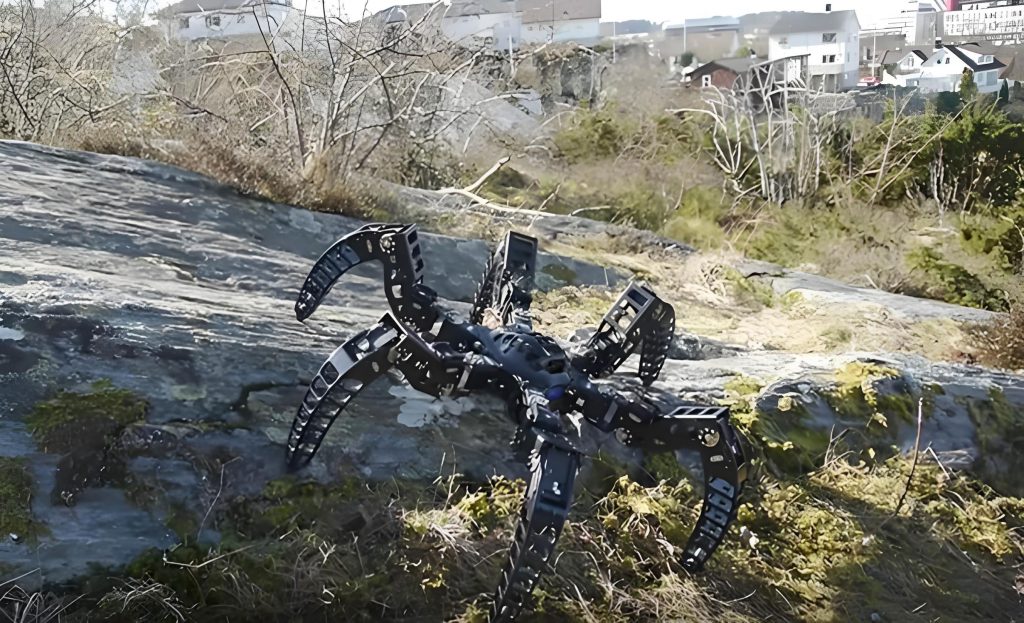
To analyze the motion of this bionic robot leg, we first establish its kinematic model. The leg consists of four links connected by rotational joints, as shown in the schematic. The joint angles are denoted as $\theta_1$, $\theta_2$, $\theta_3$, and $\theta_4$, corresponding to the root, hip, knee, and deformable joints, respectively. The link lengths are $l_1$, $l_2$, $l_3$, and $l_4$, with masses $m_1$, $m_2$, $m_3$, and $m_4$. The position of the foot tip in Cartesian coordinates can be derived using forward kinematics. For instance, if we assume the base is fixed, the foot tip position $(x, y, z)$ is given by:
$$ x = l_1 \cos(\theta_1) + l_2 \cos(\theta_1 + \theta_2) + l_3 \cos(\theta_1 + \theta_2 + \theta_3) + l_4 \cos(\theta_1 + \theta_2 + \theta_3 + \theta_4) $$
$$ y = l_1 \sin(\theta_1) + l_2 \sin(\theta_1 + \theta_2) + l_3 \sin(\theta_1 + \theta_2 + \theta_3) + l_4 \sin(\theta_1 + \theta_2 + \theta_3 + \theta_4) $$
$$ z = 0 \quad \text{(for planar motion, but can be extended to 3D)} $$
This kinematic model is essential for trajectory planning and control. To achieve smooth motion, we use B-spline interpolation for joint space trajectory generation, ensuring continuous position, velocity, and acceleration profiles. The desired foot trajectory, such as an elliptical path, is discretized into points, and inverse kinematics is applied to obtain corresponding joint angles. This approach allows the bionic robot to perform precise movements, mimicking natural locomotion patterns observed in biological systems.
For dynamics modeling, the Lagrange method is employed due to its simplicity and systematic formulation. The Lagrangian $\mathcal{L}$ is defined as the difference between kinetic energy $T$ and potential energy $V$ of the system:
$$ \mathcal{L} = T – V $$
The kinetic energy $T$ for each link involves translational and rotational components. For a link $i$ with mass $m_i$, centroidal distance $p_i$, and angular velocity $\dot{\theta}_i$, the kinetic energy is:
$$ T_i = \frac{1}{2} m_i v_i^2 + \frac{1}{2} I_i \dot{\theta}_i^2 $$
where $v_i$ is the linear velocity of the center of mass, and $I_i$ is the moment of inertia. The total kinetic energy is $T = \sum_{i=1}^4 T_i$. The potential energy $V$ is due to gravity, given by $V = \sum_{i=1}^4 m_i g h_i$, where $h_i$ is the height of the center of mass. Using the Lagrange equation:
$$ \frac{d}{dt} \left( \frac{\partial \mathcal{L}}{\partial \dot{\theta}_j} \right) – \frac{\partial \mathcal{L}}{\partial \theta_j} = \tau_j, \quad j = 1, 2, 3, 4 $$
where $\tau_j$ is the torque applied at joint $j$. This yields the dynamics equation in matrix form:
$$ \mathbf{M}(\boldsymbol{\theta}) \ddot{\boldsymbol{\theta}} + \mathbf{C}(\boldsymbol{\theta}, \dot{\boldsymbol{\theta}}) \dot{\boldsymbol{\theta}} + \mathbf{G}(\boldsymbol{\theta}) = \boldsymbol{\tau} $$
Here, $\boldsymbol{\theta} = [\theta_1, \theta_2, \theta_3, \theta_4]^T$ is the joint angle vector, $\mathbf{M}$ is the inertia matrix (symmetric and positive definite), $\mathbf{C}$ represents Coriolis and centrifugal terms, and $\mathbf{G}$ is the gravity vector. For control purposes, this model is essential but often subject to uncertainties such as unmodeled dynamics, parameter inaccuracies, and external disturbances. To address this, we develop a hybrid controller that combines model-based and adaptive elements.
The parameters used in the dynamics model are summarized in Table 1. These values are based on a prototype design of the bionic robot leg, ensuring realistic simulation scenarios.
| Link | Length (cm) | Mass (kg) | Centroid Distance (cm) |
|---|---|---|---|
| 1 | 2 | 0.1 | 2 |
| 2 | 20 | 2.0 | 10 |
| 3 | 15 | 1.5 | 7.5 |
| 4 | 10 | 1.0 | 5 |
The controller design aims to achieve accurate trajectory tracking despite model uncertainties. We propose a hybrid controller consisting of a computed torque controller for the modeled part and an RBF neural network for compensation. The computed torque controller is derived from the nominal dynamics model. If the model is perfectly known, the control law is:
$$ \boldsymbol{\tau}_0 = \mathbf{M}_0(\boldsymbol{\theta}) (\ddot{\boldsymbol{\theta}}_d + \mathbf{K}_v \dot{\mathbf{e}} + \mathbf{K}_p \mathbf{e}) + \mathbf{C}_0(\boldsymbol{\theta}, \dot{\boldsymbol{\theta}}) \dot{\boldsymbol{\theta}} + \mathbf{G}_0(\boldsymbol{\theta}) $$
where $\boldsymbol{\theta}_d$ is the desired trajectory, $\mathbf{e} = \boldsymbol{\theta}_d – \boldsymbol{\theta}$ is the tracking error, $\mathbf{K}_p$ and $\mathbf{K}_v$ are positive definite gain matrices, and $\mathbf{M}_0$, $\mathbf{C}_0$, $\mathbf{G}_0$ are nominal matrices. This yields error dynamics $\ddot{\mathbf{e}} + \mathbf{K}_v \dot{\mathbf{e}} + \mathbf{K}_p \mathbf{e} = \mathbf{0}$, ensuring global stability. However, in practice, uncertainties exist, so the actual dynamics become:
$$ \mathbf{M}(\boldsymbol{\theta}) \ddot{\boldsymbol{\theta}} + \mathbf{C}(\boldsymbol{\theta}, \dot{\boldsymbol{\theta}}) \dot{\boldsymbol{\theta}} + \mathbf{G}(\boldsymbol{\theta}) + \boldsymbol{\tau}_d = \boldsymbol{\tau} $$
where $\boldsymbol{\tau}_d$ represents disturbances. The hybrid control law is:
$$ \boldsymbol{\tau} = \boldsymbol{\tau}_0 + \boldsymbol{\tau}_c $$
with $\boldsymbol{\tau}_c = \mathbf{M}_0(\boldsymbol{\theta}) \boldsymbol{\tau}_n$, where $\boldsymbol{\tau}_n$ is the output of an RBF neural network. The RBF network approximates the uncertainty term $\boldsymbol{\Delta}$, defined as:
$$ \boldsymbol{\Delta} = \mathbf{M}_0^{-1} \left( \Delta \mathbf{M} \ddot{\boldsymbol{\theta}} + \Delta \mathbf{C} \dot{\boldsymbol{\theta}} + \Delta \mathbf{G} + \boldsymbol{\tau}_d \right) $$
where $\Delta \mathbf{M}$, $\Delta \mathbf{C}$, and $\Delta \mathbf{G}$ are modeling errors. The RBF network has an input layer with 8 neurons (joint errors and their derivatives, i.e., $\mathbf{x} = [\mathbf{e}^T, \dot{\mathbf{e}}^T]^T$), a hidden layer with 5 Gaussian basis functions, and an output layer with 4 neurons (one per joint). The output is:
$$ \boldsymbol{\tau}_n = \hat{\mathbf{W}}^T \boldsymbol{\phi}(\mathbf{x}) $$
where $\hat{\mathbf{W}}$ is the weight matrix and $\boldsymbol{\phi}$ is the basis function vector. The ideal approximation is $\boldsymbol{\Delta} = \mathbf{W}^T \boldsymbol{\phi}(\mathbf{x}) + \boldsymbol{\epsilon}$, with bounded approximation error $\boldsymbol{\epsilon}$. The weight update law uses adaptive control theory:
$$ \dot{\hat{\mathbf{W}}} = \Gamma \boldsymbol{\phi}(\mathbf{x}) \mathbf{s}^T $$
where $\Gamma$ is a positive definite matrix and $\mathbf{s} = \dot{\mathbf{e}} + \Lambda \mathbf{e}$ is a sliding surface variable. This ensures that the tracking error converges to zero despite uncertainties. The stability of the closed-loop system is proven via Lyapunov analysis. Consider the Lyapunov function candidate:
$$ V = \frac{1}{2} \mathbf{s}^T \mathbf{M}_0 \mathbf{s} + \frac{1}{2} \text{tr}(\tilde{\mathbf{W}}^T \Gamma^{-1} \tilde{\mathbf{W}}) $$
where $\tilde{\mathbf{W}} = \mathbf{W} – \hat{\mathbf{W}}$. Taking the derivative and substituting the control law, we obtain $\dot{V} \leq -\mathbf{s}^T \mathbf{K} \mathbf{s} + \eta$, where $\mathbf{K}$ is a gain matrix and $\eta$ is a bounded term due to approximation errors. Using Barbalat’s lemma, it can be shown that $\mathbf{s} \to \mathbf{0}$ as $t \to \infty$, implying asymptotic tracking. This hybrid controller effectively combines the robustness of computed torque with the adaptability of neural networks, making it suitable for real-world bionic robot applications.
To validate the controller, we conduct simulations in MATLAB. The bionic robot leg is tasked with tracking an elliptical foot trajectory, representing a typical stepping motion. The ellipse has a major axis of 10 cm (step length) and a minor axis of 5 cm (lift height), discretized into points for inverse kinematics. The joint initial conditions are $\boldsymbol{\theta}(0) = [0.6, 0.5, 0.6, 0.5]^T$ rad, with zero initial velocities and accelerations. The gain matrices are chosen as $\mathbf{K}_p = \text{diag}(100, 100, 100, 100)$ and $\mathbf{K}_v = \text{diag}(20, 20, 20, 20)$. The RBF network parameters include Gaussian widths of 0.5 and learning rate $\Gamma = 0.1$. Disturbances are modeled as random noise with amplitude 0.1 Nm to simulate real-world conditions.
The simulation results compare the performance of pure computed torque control (CTC) versus the hybrid computed torque plus RBF neural network control (CTC+RBF). Table 2 summarizes key performance metrics, including root mean square error (RMSE) and maximum error for each joint over a 30-second simulation.
| Joint | Control Method | RMSE (rad) | Max Error (rad) |
|---|---|---|---|
| 1 | CTC | 0.025 | 0.045 |
| CTC+RBF | 0.005 | 0.010 | |
| 2 | CTC | 0.030 | 0.050 |
| CTC+RBF | 0.006 | 0.012 | |
| 3 | CTC | 0.028 | 0.048 |
| CTC+RBF | 0.007 | 0.015 | |
| 4 | CTC | 0.022 | 0.040 |
| CTC+RBF | 0.004 | 0.008 |
The results clearly show that the hybrid controller reduces tracking errors significantly. For instance, joint 1 exhibits an RMSE of 0.005 rad with CTC+RBF, compared to 0.025 rad with CTC alone. This improvement is consistent across all joints, demonstrating the efficacy of neural network compensation. The deformable joint (joint 4) shows particularly low errors, highlighting its role in enhancing adaptability. The trajectory tracking plots reveal that the hybrid controller achieves convergence within 8 seconds, while the pure computed torque controller exhibits steady-state errors due to uncertainties. This underscores the importance of adaptive elements in bionic robot control, especially for legs with complex dynamics.
Further analysis involves testing the bionic robot leg under varying payload conditions to simulate different operational scenarios. By adding mass to the foot tip, we evaluate the controller’s robustness. The hybrid controller maintains stable performance, with errors increasing only slightly, whereas the pure computed torque controller shows significant degradation. This resilience is crucial for bionic robots deployed in dynamic environments where payloads may change, such as carrying tools or samples. Additionally, we simulate different terrains by introducing uneven ground profiles, requiring the leg to adjust its trajectory online. The RBF network quickly adapts to these changes, showcasing its learning capability. These simulations affirm that the proposed control strategy is well-suited for real-world bionic robot applications, where uncertainty and variability are common.
The dynamics model can be extended to include friction effects, which are often nonlinear and difficult to model accurately. For joint $j$, the friction torque $\tau_{f,j}$ can be represented as a combination of viscous and Coulomb friction:
$$ \tau_{f,j} = b_j \dot{\theta}_j + c_j \text{sgn}(\dot{\theta}_j) $$
where $b_j$ and $c_j$ are coefficients. Incorporating this into the dynamics equation, the control law can be adjusted to compensate for friction. The RBF network can learn these nonlinearities online, further improving accuracy. This adaptability is a key advantage of intelligent control systems for bionic robots, enabling them to operate efficiently in harsh conditions.
In terms of implementation, the control algorithm can be deployed on embedded systems with real-time constraints. The computational burden of the RBF network is manageable, as it involves simple matrix operations. For a bionic robot with six legs, each leg can be controlled independently using the proposed method, or coordination can be achieved through higher-level gait planning. Central pattern generators (CPGs) inspired by biological neural circuits can be integrated to produce rhythmic movements, enhancing the natural locomotion of the bionic robot. Such bio-inspired approaches align with the overarching goal of creating robots that emulate biological systems not only in structure but also in control mechanisms.
The design of the deformable joint warrants further discussion. In biological limbs, joints often have multiple degrees of freedom, allowing for complex motions. Our deformable joint adds an extra rotational axis, enabling the bionic robot leg to mimic actions like twisting or pronation. This can be beneficial for tasks such as grasping or stabilizing on slippery surfaces. The joint is actuated by a servo motor with high torque output, ensuring precise control. The kinematics of this joint are integrated into the overall model, and its dynamics are accounted for in the Lagrange formulation. This comprehensive modeling approach ensures that the bionic robot leg behaves predictably across its entire workspace.
Future work will focus on experimental validation using a physical prototype of the bionic robot. Challenges include sensor integration for feedback, such as encoders for joint angles and force sensors for ground contact. Additionally, machine learning techniques can be employed to optimize controller parameters online, reducing the need for manual tuning. Deep reinforcement learning, for instance, could enable the bionic robot to learn optimal gaits through trial and error in simulation, then transfer the policy to the real world. This would further enhance the autonomy and adaptability of bionic robots, pushing the boundaries of what is possible in robotics.
In conclusion, this paper presents a thorough dynamics analysis and control design for a hexapod bionic robot leg with a deformable joint. The Lagrange method provides a systematic dynamics model, while the hybrid computed torque and RBF neural network controller ensures robust trajectory tracking despite uncertainties. Simulations demonstrate significant performance improvements over traditional methods, validating the approach. The integration of adaptive elements is essential for bionic robots to operate in unstructured environments, and this work contributes to that goal. As robotics continues to evolve, bio-inspired designs like this will play a pivotal role in creating machines that can navigate the world with the grace and efficiency of living organisms.
The potential applications of such bionic robots are vast. In planetary exploration, they could traverse rocky terrains on Mars or the Moon, collecting samples and deploying instruments. In disaster response, they could navigate rubble to locate survivors. Underwater, they could inspect pipelines or coral reefs. The military could use them for reconnaissance in dangerous areas. Each scenario requires adaptability, which our leg design and control strategy aim to provide. By continuing to refine these technologies, we move closer to realizing the vision of versatile, autonomous bionic robots that can assist humans in challenging tasks.
From a broader perspective, the study of bionic robots bridges engineering and biology, fostering interdisciplinary innovation. Insights from biomechanics inform robot design, while control algorithms inspired by neural systems enhance performance. This synergy accelerates progress in both fields, leading to breakthroughs that benefit society. As computational power increases and materials improve, bionic robots will become more capable and affordable, opening new frontiers in automation and robotics. The journey towards truly lifelike robots is long, but each step, such as the one described here, brings us closer to that future.