
1. Introduction
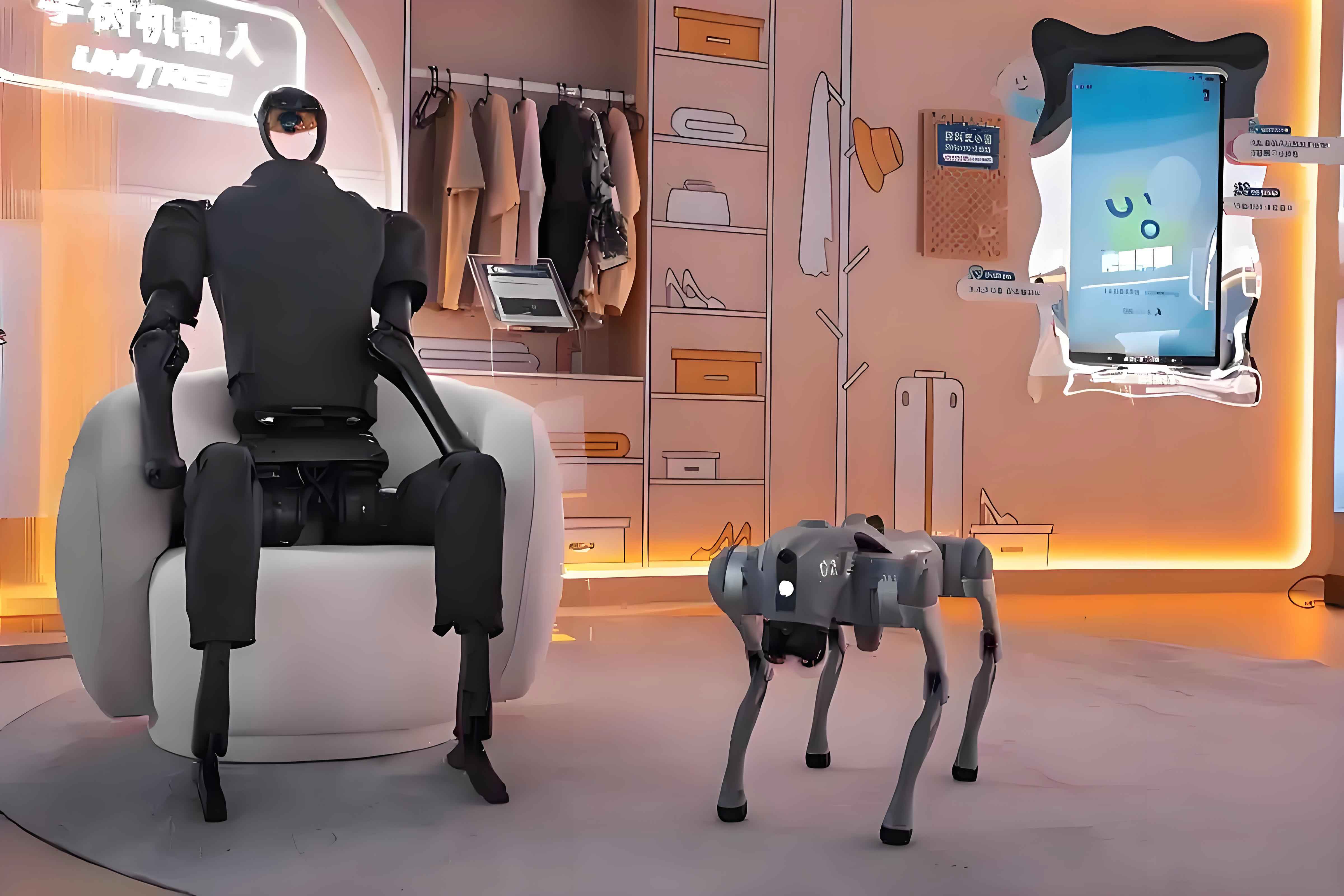
With the accelerating pace of population aging and the increasing shortage of labor in modern societies, there is a growing demand for versatile robotic systems that can operate efficiently in human-centered environments. Among all types of robots, the humanoid robot is considered one of the most promising platforms for future service, rescue, and industrial applications. The human-like morphology of a humanoid robot allows it to naturally adapt to tools, workspaces, and architectural constraints designed for humans. Unlike wheeled robots, a humanoid robot can step over obstacles, climb stairs, and traverse narrow passages by using its legs. However, achieving robust and stable locomotion in real-world indoor environments remains a challenging problem. A humanoid robot must perceive its surroundings accurately, understand semantic information, and generate appropriate footholds to maintain balance and avoid falls.
In this thesis, we focus on three fundamental problems for humanoid robots operating in indoor environments: accurate pose estimation, semantic map construction, and foothold planning for stair climbing. These problems are strongly coupled. First, the robot needs a reliable visual odometry system to estimate its own pose. Second, based on the estimated pose, the robot must build a semantic map that contains both global semantic information (e.g., objects and places) and local geometric information (e.g., elevation maps). Third, using the elevation data and the robot’s pose, the robot must plan footholds on complex terrain such as stairs and execute them with a learned control policy. To address these challenges, we propose a point-line feature based visual odometry, a hybrid semantic mapping framework, and a reinforcement learning based footstep tracking strategy for staircase locomotion.
2. Point-Line Visual Odometry for Humanoid Robots
2.1 Overall Framework
Visual odometry is the core module that provides the humanoid robot with real-time pose estimates. Our visual odometry system is built upon the ORB-SLAM3 framework but introduces line features to improve robustness in weakly textured indoor scenes and under motion blur caused by bipedal walking. The overall pipeline consists of three parallel threads: tracking, local mapping, and loop closing. The tracking thread extracts ORB point features and improved EDLines line features from RGB-D images, performs feature matching, and computes the initial camera pose. The local mapping thread performs bundle adjustment over a sliding window of keyframes, jointly optimizing point features, line features, and camera poses. The loop closing thread detects revisits and launches global optimization. The integration of line features is highlighted in the optimization modules.
2.2 Line Feature Extraction
We adopt the EDLines algorithm as the base line segment detector because of its high computational efficiency. However, the original EDLines detects segments at a single scale and tends to produce fragmented or redundant segments in complex scenes. To improve quality, we construct a Gaussian image pyramid with three layers using a scale factor of 1.2. On each layer, we run EDLines independently and then map the detected segments back to the original image resolution. This multi-scale strategy improves the scale invariance of line features and ensures that the same physical edges can be detected from different distances.
After mapping, we merge duplicate or fragmented segments based on two conditions: geometric proximity and angular similarity. Let two line segments have endpoints \(p_1, p_2\) and \(p_3, p_4\). We compute the four perpendicular distances:
\[
\begin{aligned}
d_1 &= \operatorname{dist}(p_1, \operatorname{line}(p_3, p_4)), \\
d_2 &= \operatorname{dist}(p_2, \operatorname{line}(p_3, p_4)), \\
d_3 &= \operatorname{dist}(p_3, \operatorname{line}(p_1, p_2)), \\
d_4 &= \operatorname{dist}(p_4, \operatorname{line}(p_1, p_2)).
\end{aligned}
\]
If \(\min(d_1,d_2,d_3,d_4) < 5\) pixels and the angle between the two directional vectors is less than \(10^\circ\), the two segments are merged. The merged segment is determined by projecting all four endpoints onto the average direction and selecting the two extreme projected points. Finally, we discard segments shorter than 40 pixels to retain only stable and representative features.
Table 2.1 compares the performance of the original LSD, the original EDLines, and our improved EDLines on a typical indoor frame.
| Algorithm | Average segment length (pixels) | Computation time (ms) |
|---|---|---|
| LSD | 35.36 | 29.87 |
| EDLines | 76.45 | 10.24 |
| Improved EDLines | 105.38 | 18.31 |
2.3 Line Feature Matching
To match line features efficiently, we propose a projection-based matching method that combines geometric constraints and LBD descriptor scores. Each observed line segment is represented by its normal vector \(\mathbf{n} = [n_x, n_y]^T\) and the distance \(h\) to the image origin, satisfying:
\[
\mathbf{n}^T \mathbf{u} – h = 0,
\]
where \(\mathbf{u}\) is an arbitrary point on the line. We create a two-dimensional hash grid indexed by the normal angle \(\theta = \arctan(n_y / n_x)\) and the distance \(h\). The grid resolutions are \(\Delta\theta = 10^\circ\) and \(\Delta h = 100\) pixels.
Given the predicted camera pose from the constant velocity model, we project line features from the previous frame or the local map into the current frame. The projected line normal and distance are computed as:
\[
\mathbf{n}’ = \mathbf{R}_{k} \mathbf{n}_{k-1}, \qquad h’ = h_{k-1} + \mathbf{t}_k^T \mathbf{n}_{k-1},
\]
where \(\mathbf{R}_k\) and \(\mathbf{t}_k\) are the rotation and translation of the current camera pose. The projected line falls into a hash bin. Within the same bin, we compute the Hamming distance between LBD descriptors and the point-to-line distance between projected endpoints and candidate segments. The best match must satisfy a ratio test on the descriptor distance and a distance threshold on the line-to-line gap.
To further improve robustness under blur, we compared feature matching statistics between a static robot and a walking humanoid robot. The results are shown in Table 2.2.
| Condition | Number of matched point features | Number of matched line features |
|---|---|---|
| Static (clear image) | 309 | 31 |
| Walking (blurred image) | 115 | 23 |
2.4 Nonlinear Optimization with Line Features
Our optimization framework minimizes a combination of point reprojection errors and line reprojection errors. We define both a 2D line reprojection error and a 3D line reprojection error. The 3D error is used when depth information is available for the line segment endpoints.
For a 3D line \(\mathbf{L}\) with endpoints \(\mathbf{P}_W\) and \(\mathbf{Q}_W\), the 2D reprojection error is computed by projecting the endpoints into the image plane and measuring the distances to the observed line segment \(\mathbf{l}\). Let the observed line be represented by its normal \(\mathbf{n}_l\) and distance \(h_l\). The error is:
\[
\mathbf{e}_{2D} =
\begin{bmatrix}
d_{D}(\gamma(\mathbf{K}\mathbf{T}\mathbf{P}_W), \mathbf{l}) \\
d_{D}(\gamma(\mathbf{K}\mathbf{T}\mathbf{Q}_W), \mathbf{l})
\end{bmatrix},
\]
where \(\gamma([u,v,w]^T) = [u/w, v/w]^T\) is the perspective projection operator, \(\mathbf{K}\) is the camera intrinsic matrix, and \(\mathbf{T}\) is the camera pose. The point-to-line distance in 2D is \(d_D(\mathbf{x}, \mathbf{l}) = \mathbf{n}_l^T \mathbf{x} – h_l\).
The 3D line reprojection error is defined by back-projecting the observed 2D line into 3D space. Let \(\mathbf{P}_C’\) and \(\mathbf{Q}_C’\) be the back-projected endpoints using the depth values \(\delta_p\) and \(\delta_q\):
\[
\mathbf{P}_C’ = \mathbf{K}^{-1} \tilde{\mathbf{p}} \delta_p, \qquad
\mathbf{Q}_C’ = \mathbf{K}^{-1} \tilde{\mathbf{q}} \delta_q.
\]
Then the 3D error for the 3D point \(\mathbf{P}_C\) with respect to the back-projected line is:
\[
d_{3D}(\mathbf{P}_C, \mathbf{L}’) = \frac{\|(\mathbf{P}_C – \mathbf{P}_C’) \times (\mathbf{P}_C – \mathbf{Q}_C’)\|}{\|\mathbf{P}_C’ – \mathbf{Q}_C’\|} + \mu \|\mathbf{P}_C – \mathbf{P}_C’\|,
\]
where \(\mu \in [0,1]\) balances the point-to-line distance and the endpoint distance. The full line error vector is:
\[
\mathbf{e}_{3D} =
\begin{bmatrix}
d_{3D}(\mathbf{P}_C, \mathbf{L}’) \\
d_{3D}(\mathbf{Q}_C, \mathbf{L}’)
\end{bmatrix}.
\]
The total objective function for the optimization includes point errors, 2D line errors, and 3D line errors:
\[
E = \sum_{k \in \mathcal{K}} \left( \sum_{i \in \mathcal{P}_k} \rho(\mathbf{e}_{2D}^{p}(i,k)) + \sum_{j \in \mathcal{L}_k} \rho(\mathbf{e}_{2D}^{l}(j,k)) + \sum_{r \in \mathcal{L}_k^d} \rho(\mathbf{e}_{3D}(r,k)) \right),
\]
where \(\mathcal{P}_k\), \(\mathcal{L}_k\), and \(\mathcal{L}_k^d\) are the sets of points, all lines, and depth-valid lines observed in keyframe \(k\), respectively, and \(\rho\) is a robust loss function. The Levenberg-Marquardt algorithm is used to solve the resulting nonlinear least squares problem.
2.5 Experimental Evaluation on TUM Dataset
We evaluated the proposed point-line visual odometry on multiple TUM RGB-D sequences. Table 2.3 reports the absolute trajectory error (ATE) root mean square error (RMSE) compared with the point-feature-only ORB-SLAM3.
| Sequence | Proposed VO | ORB-SLAM3 | Improvement |
|---|---|---|---|
| Fr1_360 | 0.1096 | 0.1979 | 0.0883 |
| Fr1_desk | 0.0166 | 0.0169 | 0.0003 |
| Fr1_plant | 0.0217 | 0.0147 | -0.0070 |
| Fr1_rpy | 0.0174 | 0.0215 | 0.0042 |
| Fr2_dishes | 0.0314 | 0.0424 | 0.0110 |
| Fr2_desk | 0.0123 | 0.0085 | -0.0038 |
| Fr2_metallic | 0.1426 | 0.2165 | 0.0739 |
| Fr2_rpy | 0.0033 | 0.0032 | 0.0001 |
The results show that the proposed point-line VO significantly improves accuracy in challenging sequences with fast motion and weak texture, such as Fr1_360 and Fr2_metallic. In sequences where ORB-SLAM3 already performs well, the improvement is minor but not harmful. The line features provide supplementary geometric constraints when point features are scarce or unreliable.
3. Semantic Map Construction for Humanoid Robots
3.1 Overview
Building a semantic map is essential for a humanoid robot to understand its environment and execute high-level tasks. We propose a semantic mapping framework that integrates both global semantic information and local geometric information. The global map contains an object layer and a place layer. The object layer stores object instances with their semantic labels, sizes, and positions. The place layer segments the environment into rooms and assigns semantic categories such as corridor, bedroom, or office. In addition, we construct a local elevation map around the robot to support footstep planning and locomotion control.
3.2 Point Cloud Generation and Fusion
We use the pinhole camera model to transform depth images into organized point clouds. Given the camera intrinsic matrix \(\mathbf{K}\) and the depth value \(Z = D(u,v)\), the 3D point in the camera coordinate frame is:
\[
\begin{bmatrix} X \\ Y \\ Z \end{bmatrix} =
\begin{bmatrix}
\frac{(u – c_x) Z}{f_x} \\
\frac{(v – c_y) Z}{f_y} \\
Z
\end{bmatrix}.
\]
Then, using the camera pose \(\mathbf{T}_{CW} = [\mathbf{R}_{CW} | \mathbf{t}_{CW}]\) from the visual odometry, we transform the point cloud into the world frame:
\[
\mathbf{P}_W = \mathbf{R}_{CW}^{-1}(\mathbf{P}_C – \mathbf{t}_{CW}).
\]
To fuse a new keyframe point cloud with the global map, we first apply a statistical outlier removal filter. Then, for each point in the current point cloud, we search for a corresponding point in the map that satisfies two conditions: the Euclidean distance between the two points is below a threshold \(\varepsilon\), and the two points project to the same pixel in the keyframe. If a match is found, we update the depth value using a weighted average:
\[
d_{\mathrm{fusion}} = \frac{k-1}{k} d_{\mathrm{previous}} + \frac{1}{k} d_{\mathrm{current}},
\]
where \(k\) is the number of historical observations. The fusion weight is defined as:
\[
\alpha = \frac{d_{\mathrm{fusion}} – d_{\mathrm{previous}}}{d_{\mathrm{current}} – d_{\mathrm{previous}}},
\]
and the fused point coordinates are:
\[
\mathbf{x}_{\mathrm{fusion}} = \alpha \mathbf{x}_{\mathrm{previous}} + (1-\alpha) \mathbf{x}_{\mathrm{current}}.
\]
Finally, a voxel grid filter is applied to reduce redundancy and maintain a uniform point density.
3.3 Object-Level Semantic Extraction and Data Association
We use the FCAF3D detector, a fully convolutional anchor-free 3D object detection network trained on ScanNet, to extract object semantics from the point cloud. The detector outputs object category, 3D bounding box, and orientation for 18 common indoor object classes such as bed, table, sofa, chair, and refrigerator.
To integrate the detected objects into the global map, we associate each new observation with existing map objects. We build a 3D Intersection-over-Union (IoU) matrix between the new observations and the map objects. The 3D IoU between two bounding boxes \(A\) and \(B\) is:
\[
\operatorname{IoU}_{3D} = \frac{\operatorname{Area}_{\mathrm{overlap}} \times h_{\mathrm{overlap}}}{\operatorname{Area}_A h_A + \operatorname{Area}_B h_B – \operatorname{Area}_{\mathrm{overlap}} \times h_{\mathrm{overlap}}},
\]
where \(\operatorname{Area}_A\) and \(\operatorname{Area}_B\) are the ground-projected areas, and \(h_A, h_B\) are the heights. The overlap area and overlap height are computed from the axis-aligned bounding boxes. We then use the Hungarian algorithm to find the optimal assignment that maximizes the total IoU. Unmatched new observations are treated as new objects and added to the map. To prevent the map from storing stale objects, we periodically remove objects that have not been updated for a long time and have low successful match counts.
3.4 Spatial Segmentation via Generalized Voronoi Diagrams
To segment the indoor space into rooms, we construct a Generalized Voronoi Diagram (GVD) from the Euclidean Signed Distance Field (ESDF) of the environment. The GVD skeleton represents the topological structure of free space. We first generate a sparse graph from the GVD by removing surface points and thin structures. Then we perform a sequence of inflation operations on the ESDF. In the sparse graph, each node stores its distance to the nearest obstacle. Inflation is equivalent to reducing this distance by the inflation radius. When the radius grows, nodes with negative distances are removed, and the sparse graph splits into several connected components. Each connected component corresponds to a separate region that can be interpreted as a room.
The number of rooms is estimated as the median number of connected components over five inflation radii in the range \([0.4, 1.2]\) meters. The nodes of each connected component are clustered into a room node, and the spatial extent of the room can be inferred from the positions of these nodes. To connect the object layer and the place layer, we associate each object observation with the nearest skeleton node. Since each skeleton node belongs to a room, the object is implicitly assigned to that room.
3.5 Room Semantic Classification with Support Vector Machine
We train a support vector machine (SVM) to classify the semantic category of each room based on the objects observed inside it. The feature vector for a room is extracted from the presence of object categories. Let the global object vocabulary be \(\mathcal{O} = \{o_1, o_2, \dots, o_M\}\). For room \(i\), the binary feature vector is:
\[
\mathbf{x}_i = [x_{i1}, x_{i2}, \dots, x_{iM}], \qquad x_{ij} \in \{0, 1\}.
\]
To improve classification accuracy, we perform feature selection using mutual information (MI):
\[
\operatorname{MI}(o_j, y) = \sum_{x_{ij} \in \{0,1\}} \sum_{y} P(x_{ij}, y) \log \frac{P(x_{ij}, y)}{P(x_{ij}) P(y)},
\]
where \(y\) is the room type. Objects with low MI are removed because they appear across many room types and provide little discriminative information. Then, instead of raw presence, we compute TF-IDF weights for the remaining objects:
\[
\operatorname{TF}(o_j, \mathbf{x}_i) = \frac{N_{o_j, \mathbf{x}_i}}{N_{\mathbf{x}_i}}, \qquad
\operatorname{IDF}(o_j) = \log \frac{N_{\mathrm{total}}}{1 + N_{o_j}},
\]
\[
\operatorname{TFIDF}(o_j, \mathbf{x}_i) = \operatorname{TF}(o_j, \mathbf{x}_i) \cdot \operatorname{IDF}(o_j).
\]
The SVM is trained using a Gaussian radial basis function kernel:
\[
K(\mathbf{x}_i, \mathbf{x}_j) = \exp\left( -\frac{\|\mathbf{x}_i – \mathbf{x}_j\|^2}{2\sigma^2} \right),
\]
with \(C=1.0\). We use the one-vs-one strategy for multi-class classification and aggregate votes to predict the room label.
We evaluated the classifier on 7000 ScanNet samples with five room categories: bathroom, bedroom, dining room, hallway, and office. Table 3.1 shows the precision, recall, and F1-score for each class.
| Class | Precision | Recall | F1-score |
|---|---|---|---|
| bathroom | 0.92 | 0.88 | 0.90 |
| bedroom | 0.86 | 0.90 | 0.88 |
| dining room | 0.79 | 0.68 | 0.73 |
| hallway | 0.83 | 0.83 | 0.83 |
| office | 0.78 | 0.72 | 0.75 |
The high F1 scores for bathroom and bedroom are due to the presence of highly discriminative objects such as toilets and beds. The lower scores for dining room and office are expected because desks and chairs appear frequently in both classes.
3.6 Local Elevation Map
For a humanoid robot, the local terrain under its feet must be known with high precision to plan stable footholds. We construct a robot-centric elevation map on a multi-layer grid. Each cell stores the height estimate \(\hat{h}\), the height variance \(\hat{\sigma}_h^2\), and additional horizontal variance components \(\hat{\sigma}_x^2\) and \(\hat{\sigma}_y^2\).
A new depth measurement \(\mathbf{p}_S\) in the sensor frame is projected into the elevation map using the sensor-to-map transform:
\[
\mathbf{p}_M = \mathbf{C}_{SM} (\mathbf{p}_S – \mathbf{t}_{SM}),
\]
where \(\mathbf{C}_{SM}\) and \(\mathbf{t}_{SM}\) are the rotation and translation between the sensor and map frames. The height measurement is \(Z\), and its uncertainty is propagated from the sensor noise and the robot pose uncertainty:
\[
\sigma_z^2 = \mathbf{J}_p \mathbf{\Sigma}_S \mathbf{J}_p^T + \mathbf{J}_q \mathbf{\Sigma}_{P,q} \mathbf{J}_q^T,
\]
with Jacobians \(\mathbf{J}_p = \mathbf{P} \mathbf{C}_{SM}\) and \(\mathbf{J}_q = \mathbf{P} \mathbf{C}_{SM} [\mathbf{p}_S]_{\times}\), where \(\mathbf{P} = [0,0,1]\).
We fuse the new measurement with the existing map estimate using a Kalman filter update:
\[
\hat{h}^{+} = \frac{\sigma_z^2 \hat{h}^{-} + \hat{\sigma}_{h^{-}}^2 z}{\hat{\sigma}_{h^{-}}^2 + \sigma_z^2}, \qquad
\hat{\sigma}_{h^{+}}^2 = \frac{\hat{\sigma}_{h^{-}}^2 \sigma_z^2}{\hat{\sigma}_{h^{-}}^2 + \sigma_z^2}.
\]
When the robot moves, the map frame moves with the robot, but the terrain is fixed in the inertial frame. We update the stored variances by propagating the change in the robot pose uncertainty:
\[
\begin{bmatrix} \hat{\sigma}_x^2 \\ \hat{\sigma}_y^2 \\ \hat{\sigma}_h^2 \end{bmatrix}^{+}
=
\begin{bmatrix} \hat{\sigma}_x^2 \\ \hat{\sigma}_y^2 \\ \hat{\sigma}_h^2 \end{bmatrix}^{-}
+ \mathbf{J}_r (\mathbf{\Sigma}_P^k – \mathbf{\Sigma}_P^{k-1}) \mathbf{J}_r^T + \mathbf{J}_q (\mathbf{\Sigma}_P^k – \mathbf{\Sigma}_P^{k-1}) \mathbf{J}_q^T,
\]
where \(\mathbf{J}_r\) and \(\mathbf{J}_q\) are Jacobians of the map point with respect to the robot position and orientation.
We built local elevation maps in two real stair environments. The resolution is 0.01 m/cell. The results showed that the geometric features of the stairs, including height, depth, and boundaries, were accurately reconstructed. The elevation map provides the humanoid robot with the necessary terrain information for foothold planning.
4. Foothold Planning for Humanoid Robots
4.1 Overall Framework
The complete foothold planning and tracking framework is illustrated conceptually. First, the visual odometry module estimates the robot pose from RGB-D images. Then, the local elevation map is constructed using the depth images and the estimated pose. The elevation map is fed into the foothold planner, which generates a desired foothold sequence for the upcoming steps. The desired footholds, along with terrain height data and the robot’s proprioceptive state, are passed as observations to a reinforcement learning policy. The policy outputs joint position commands for all degrees of freedom of the humanoid robot.
4.2 Foothold Generation Using 3D-LIPM
We extend the classical three-dimensional linear inverted pendulum model (3D-LIPM) to staircase terrain. The 3D-LIPM equation of motion is:
\[
\ddot{\mathbf{r}} = \omega_0^2 (\mathbf{r} – \mathbf{p}),
\]
where \(\mathbf{r}\) is the center of mass (COM) position, \(\mathbf{p}\) is the foothold position, and \(\omega_0 = \sqrt{g/z_0}\) is the natural frequency of the pendulum. The instantaneous capture point (ICP) is defined as:
\[
\boldsymbol{\xi} = \mathbf{r} + \frac{\dot{\mathbf{r}}}{\omega_0}.
\]
The evolution of the ICP over one step of duration \(T\) is:
\[
\boldsymbol{\xi}(T) = \boldsymbol{\xi}(0) e^{\omega_0 T} + \mathbf{p} (1 – e^{\omega_0 T}).
\]
Given the desired walking velocity \(\mathbf{v} = [v_x, v_y]\) and step duration \(T_s\), the desired step length \(s_d\) and step width \(w_d\) are:
\[
s_d = |\mathbf{v}| T_\delta, \qquad w_d = \frac{w_c}{T_s} T_\delta,
\]
where \(T_\delta = T_s – t\) is the remaining time, and \(w_c\) is a commanded lateral offset. The offset between the predicted ICP and the desired foothold is computed as:
\[
\mathbf{b} =
\begin{bmatrix}
\frac{s_d + (\xi_y – p_y) – \xi_x}{e^{\omega_0 T_\delta} – 1} \\
\frac{w_d / 2 – \xi_y + p_y}{e^{\omega_0 T_\delta} – 1}
\end{bmatrix}.
\]
Then the desired foothold is:
\[
\hat{\mathbf{p}} =
\begin{bmatrix}
\xi_x – b_x \\
\xi_y + (-1)^n b_y
\end{bmatrix},
\]
where \(n\) is the step index (even for left, odd for right). For turning, we rotate the offset vector by the yaw angle \(\theta = \arctan(v_y/v_x)\).
4.3 Staircase Foothold Adaptation
On stairs, the foothold positions must be constrained to lie on the step surfaces. We define the feasible region for foothold \(p\) in the x-direction as:
\[
p_x \in \left[ k d_{\mathrm{step}} + \tau_1, \; k d_{\mathrm{step}} + \tau_2 \right],
\]
where \(k\) is the step index, \(d_{\mathrm{step}}\) is the step depth, and \(\tau_1, \tau_2\) are safety margins related to the robot’s foot dimensions. In the y-direction, the foothold must satisfy:
\[
p_y \in \left[ -w_{\mathrm{step}}/2, \; w_{\mathrm{step}}/2 \right].
\]
We also adjust the step length when the robot crosses a stair edge. Let \(h_{\mathrm{step}}\) be the step height. The modified step length is:
\[
s_d =
\begin{cases}
|\mathbf{v}| T_\delta \left(1 – \alpha (h_{\mathrm{step}} – 0.15) / 0.15 \right), & h_{\mathrm{step}} > 0.15 \text{ m}, \\
|\mathbf{v}| T_\delta, & h_{\mathrm{step}} \leq 0.15 \text{ m}.
\end{cases}
\]
For each stair, the number of footholds depends on the step depth \(d_{\mathrm{step}}\) and the robot foot length \(l_{\mathrm{foot}}\). If \(d_{\mathrm{step}} – l_{\mathrm{foot}} > k\) and \(s_d < d_{\mathrm{step}} – k\), we place a single foothold per stair; otherwise we place multiple footholds. For single-foothold cases, we set the step length equal to the depth of the stair:
\[
s_d = d_{\mathrm{step}}.
\]
To avoid the robot’s toe hitting the riser, we choose the front safety margin \(\tau_2\) larger than the rear margin \(\tau_1\). This conservative setting ensures that the foot is fully supported on the stair even if the heel is slightly off the edge.
4.4 Reinforcement Learning for Foothold Tracking
We train a neural network policy using Proximal Policy Optimization (PPO) to track the desired footholds while maintaining stability on stairs. The policy maps observations to target joint positions. The overall objective is to maximize:
\[
J(\pi_{\theta}) = \mathbb{E}_{\tau \sim \pi_{\theta}} \left[ \sum_{t=0}^{T} \gamma^t R_t \right].
\]
PPO clips the probability ratio to ensure stable updates:
\[
L^{\mathrm{CLIP}}(\theta) = \mathbb{E}_t \left[ \min\left( r_t(\theta) A_t, \; \operatorname{clip}(r_t(\theta), 1-\epsilon, 1+\epsilon) A_t \right) \right],
\]
where \(r_t(\theta) = \pi_{\theta}(a_t|s_t) / \pi_{\theta_{\mathrm{old}}}(a_t|s_t)\), \(A_t\) is the advantage estimate, and \(\epsilon = 0.2\).
4.4.1 State and Action Spaces
The action space contains the target positions of all 29 joints of the humanoid robot: 14 arm joint positions, 12 leg joint positions, and 3 waist joint positions. The state space is designed to provide sufficient information for the policy while keeping the dimensionality manageable. It includes:
- Terrain height map: an \(11 \times 17 = 187\) dimensional local elevation map around the robot with a resolution of 0.1 m/cell.
- Desired foothold position: the 3D coordinates of the next target foothold.
- Joint positions and velocities for all 29 joints.
- Base angular velocity (3 values) and base linear velocity (3 values).
- Projected gravity direction (3 values), which indicates body orientation.
- The previous action output (29 values) to smooth transitions and reduce partial observability.
Table 4.1 summarizes the state space dimensions.
| State component | Source | Dimension |
|---|---|---|
| Terrain height | Elevation map | 187 |
| Foothold position | Foothold planner | 3 |
| Arm joint positions | Encoders | 14 |
| Leg joint positions | Encoders | 12 |
| Waist joint positions | Encoders | 3 |
| Arm joint velocities | Encoders | 14 |
| Leg joint velocities | Encoders | 12 |
| Waist joint velocities | Encoders | 3 |
| Base angular velocity | IMU | 3 |
| Base linear velocity | State estimator | 3 |
| Projected gravity | IMU | 3 |
| Previous action | History | 29 |
| Total | 286 |
4.4.2 Reward Function
The reward function is crucial for guiding the policy toward stable stair climbing. We design the total reward as the sum of several terms:
\[
R = R_{\mathrm{foothold}} + R_{\mathrm{timing}} + R_{\mathrm{force}} + R_{\mathrm{action}} + R_{\mathrm{energy}} + R_{\mathrm{velocity}} + R_{\mathrm{torque}} + R_{\mathrm{limit}} + R_{\mathrm{termination}}.
\]
The foothold tracking reward is:
\[
R_{\mathrm{foothold}} = \alpha_l \exp\left( -\frac{\|\hat{\mathbf{p}} – \mathbf{p}_{\mathrm{actual}}\|^2}{\sigma_l^2} \right),
\]
where \(\hat{\mathbf{p}}\) is the desired foothold position and \(\mathbf{p}_{\mathrm{actual}}\) is the actual foot position at landing. This reward encourages the robot to place its feet accurately on the planned footholds.
The timing reward encourages the robot to step within the prescribed step duration:
\[
R_{\mathrm{timing}} = \alpha_t \exp\left( -\frac{(t – T_s)^2}{\sigma_t^2} \right).
\]
The impact force reward penalizes large ground reaction forces to protect the mechanical structure:
\[
R_{\mathrm{force}} = -\alpha_f \max(0, |F| – F_{\max}),
\]
where \(F\) is the measured impact force and \(F_{\max}\) is the allowed maximum. The action smoothness reward penalizes large changes in consecutive actions:
\[
R_{\mathrm{action}} = -\alpha_a \sum_k |a_k – a_{k-1}|.
\]
The energy reward encourages the robot to minimize joint torques:
\[
R_{\mathrm{energy}} = -\alpha_e \sum_n |\tau_n|.
\]
The velocity tracking reward keeps the robot moving at the commanded speed:
\[
R_{\mathrm{velocity}} = -\alpha_v \|\hat{\mathbf{v}} – \mathbf{v}\|.
\]
Joint torque and position limits are penalized to prevent hardware damage:
\[
R_{\mathrm{torque}} = -\alpha_{\tau} \max(0, |\tau| – \tau_{\max}), \qquad
R_{\mathrm{limit}} = -\alpha_q \max(0, |q| – q_{\max}).
\]
Finally, a large negative reward is applied if the episode terminates due to a fall:
\[
R_{\mathrm{termination}} =
\begin{cases}
\alpha_d, & \text{if termination}, \\
0, & \text{otherwise}.
\end{cases}
\]
4.5 Training Setup
We trained the policy in NVIDIA Isaac Gym with 4096 parallel environments on a single GPU. The humanoid robot model was simulated with accurate link masses, inertias, and joint limits. We used curriculum learning to incrementally increase stair height and decrease step depth. The PPO hyperparameters are listed in Table 4.2.
| Hyperparameter | Value |
|---|---|
| Clip ratio \(\epsilon\) | 0.2 |
| Learning rate | \(1 \times 10^{-3}\) |
| Discount factor \(\gamma\) | 0.99 |
| Entropy coefficient | 0.01 |
| Number of parallel envs | 4096 |
| Total iterations | 10000 |
4.6 Experimental Results
4.6.1 Simulation Results
We evaluated the trained policy in two simulated stair environments. The first environment had stairs with height 0.15 m and depth 0.40 m. The second environment had stairs with height 0.15 m and depth 0.20 m. The robot walked at a commanded speed of 0.5 m/s. In the first environment, the robot placed two footholds on each stair, alternating left and right. In the second environment, the robot placed a single foothold on each step, which is consistent with the planning algorithm. The tracking errors between the actual foot positions and the desired footholds were measured. The results show that the robot accurately tracked the planned footholds in both environments. Some deviations were observed when the robot’s toe slightly collided with the riser, but the policy compensated via joint adjustments and maintained balance throughout the climb.
4.6.2 Real-world Experiments
Real-world experiments were conducted on the Unitree G1 humanoid robot. Two staircases with parameters identical to the simulation environments were selected. The robot walked at 0.5 m/s. In the first environment, the robot successfully climbed the stairs by placing two feet on each step. In the second environment, the robot climbed with a single foot per step. We manually measured the actual foothold positions after each run. Tables 4.3 and 4.4 list the absolute tracking errors in the \(x\) and \(y\) directions for the two scenarios.
| Foothold index | 1 | 2 | 3 | 4 | 5 | 6 | 7 |
|---|---|---|---|---|---|---|---|
| \(x\)-error (cm) | 1 | 2 | 1 | 3 | 1 | 2 | 1 |
| \(y\)-error (cm) | 1 | 1 | 1 | 6 | 4 | 6 | 8 |
| Foothold index | 1 | 2 | 3 | 4 |
|---|---|---|---|---|
| \(x\)-error (cm) | 1 | 2 | 2 | 2 |
| \(y\)-error (cm) | 1 | 1 | 3 | 3 |
In the first scenario, the larger errors in the later steps were mainly caused by the slippery surface of the stairs, which resulted in slight foot slippage during weight transfer. In the second scenario, the errors were within an acceptable range. These experiments demonstrate that the proposed foothold planning and tracking approach enables a humanoid robot to climb stairs reliably under different stair geometries.
5. Conclusion
In this thesis, we studied semantic mapping and footstep planning for humanoid robots in indoor environments. We first improved the robustness of visual odometry by integrating line features into the ORB-SLAM3 pipeline. An improved EDLines algorithm was proposed for multi-scale line extraction, and a projection-based matching method was developed to efficiently associate line features. We derived both 2D and 3D line reprojection errors and integrated them into the nonlinear optimization backend. Experiments on TUM datasets showed that the proposed point-line visual odometry outperforms the point-only system in weak-texture and fast-motion sequences.
Second, we proposed a semantic mapping framework that builds a global map with object instances and room-level semantic labels. Object semantics are extracted by FCAF3D and fused into the map using 3D IoU matching and the Hungarian algorithm. Room segmentation is achieved by inflating a GVD skeleton until the graph splits into connected components. A TF-IDF weighted SVM classifies the room type from the observed objects. In addition, a local elevation map is constructed to provide geometric detail for locomotion planning. Real-world experiments demonstrated that the proposed framework can build accurate semantic maps of indoor scenes.
Finally, we developed a foothold planning method for stair climbing. The planner extends the 3D-LIPM model to handle stair constraints and generates feasible foothold positions. We then trained a PPO-based tracking policy that maps terrain height, desired footholds, and proprioceptive states to joint commands. Simulation and real-world experiments on the G1 humanoid robot confirmed that the robot can climb stairs with varying depths by either placing one or two footholds per step. The successful deployment highlights the importance of combining geometric perception, semantic understanding, and learning-based control for humanoid robots operating in complex indoor environments.
There are several directions for future work. First, the visual odometry could be coupled with leg odometry or inertial sensors to further reduce drift during dynamic walking. Second, the semantic map could be used for higher-level task planning and human-robot interaction. Third, the foothold planner can be extended to other challenging terrain such as rubble, slopes, and gaps. Ultimately, the integration of semantic perception and locomotion control will enable humanoid robots to operate autonomously in unstructured human environments.