
Simultaneous Localization and Mapping (SLAM) is a fundamental capability for embodied robots operating in unknown environments. Unlike wheeled or tracked platforms, humanoid robots possess a bipedal structure that enables them to navigate in complex terrains such as stairs, ramps, and cluttered indoor spaces. However, the unique kinematics and dynamics of humanoid robots pose significant challenges for sensor fusion, state estimation, and dense mapping. In this work, I present a comprehensive study on SLAM methods tailored for embodied robots, focusing on robust targetless LiDAR-camera calibration, a 3D Gaussian Splatting (3DGS) based multi-sensor SLAM system, and the deployment on a custom-built small humanoid robot. The proposed methods extensively exploit complementary sensor information from LiDAR, cameras, and inertial measurement units (IMUs) to achieve accurate localization and high-fidelity map reconstruction. Through extensive experiments in both indoor and outdoor scenarios, including sensor-degraded conditions, the proposed approaches demonstrate superior performance compared to state-of-the-art methods.
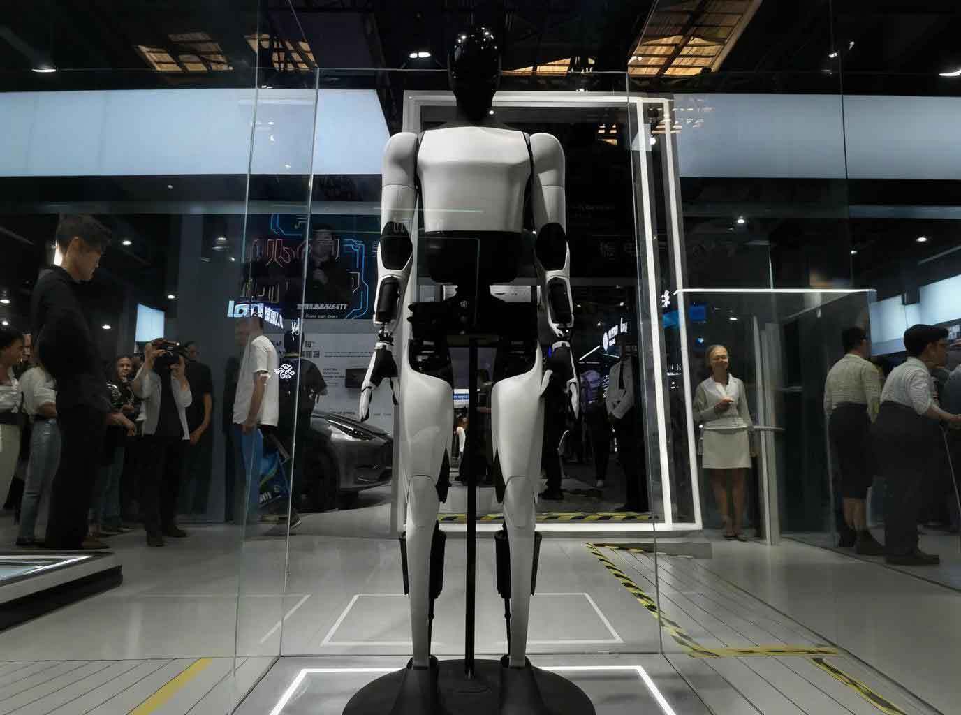
The rest of this article is organized as follows. Section 2 reviews related work on multi-sensor fusion SLAM and humanoid robotics. Section 3 introduces a targetless LiDAR-camera calibration method based on intensity and geometric edge features. Section 4 presents a 3DGS-based SLAM system that tightly integrates LiDAR, camera, and IMU measurements. Section 5 describes the design and implementation of a small humanoid robot platform and its application to autonomous localization and dense mapping. Finally, Section 6 concludes the work and discusses future directions.
1. Introduction
Embodied robots are expected to interact with the physical world in real time, which requires not only accurate self-localization but also rich semantic and geometric understanding of the surroundings. Traditional SLAM systems, such as ORB-SLAM and LOAM, typically produce sparse or semi-dense maps that are insufficient for downstream tasks like navigation, manipulation, and scene understanding. Recent advances in neural rendering and explicit 3D representations have opened new avenues for dense, photorealistic mapping. Among them, 3D Gaussian Splatting (3DGS) has emerged as a powerful technique that combines high rendering quality with real-time performance, making it particularly attractive for embodied robot applications.
However, integrating 3DGS into a SLAM framework for humanoid robots is nontrivial. Humanoid robots experience frequent vibrations, abrupt accelerations, and complex foot-ground interactions, which can cause sensor extrinsic parameters to drift over time. Moreover, the operating environments may vary from indoor office scenes to wide outdoor areas, introducing challenges such as sparse depth, illumination changes, and dynamic objects. To address these issues, I propose a multi-sensor fusion approach that leverages the strengths of LiDAR, camera, and IMU simultaneously. The key idea is to use a fast point-cloud-based odometry to obtain an initial pose estimate, then refine it using gradient losses derived from rendered and real color/depth images. The refined pose is used to update a 3DGS map, which is continuously optimized to achieve both geometric accuracy and visual realism.
2. Related Work
2.1 Multi-Sensor Fusion SLAM
Numerous SLAM systems have been developed for mobile robots. Pure visual methods like VINS-Mono and ORB-SLAM3 are low-cost but suffer from illumination changes and textureless areas. LiDAR-based methods such as LOAM and Fast-LIO2 provide accurate geometric measurements but lack color information and are vulnerable in degenerate scenes like long corridors. Recent systems such as LVI-SAM and FAST-LIVO tightly fuse visual, inertial, and LiDAR data to achieve robust state estimation. For embodied robots, the sensor suite must be compact and lightweight, often including a small solid-state LiDAR, a depth camera, and an IMU. This configuration motivates the development of efficient and robust extrinsic calibration and fusion algorithms.
2.2 3D Gaussian Splatting for SLAM
The use of neural implicit representations in SLAM has been explored extensively. iMAP and NICE-SLAM use MLPs, while Point-SLAM and Co-SLAM adopt point-based or hybrid representations. More recently, 3DGS has been adopted in several SLAM systems such as SplaTAM, MonoGS, and GS-SLAM. These methods demonstrate that 3DGS can provide high-fidelity reconstruction and real-time rendering. However, most existing 3DGS-SLAM systems rely on RGB-D cameras and are limited to small indoor scenes. In contrast, the proposed method combines LiDAR-inertial odometry with 3DGS rendering to handle larger and more complex environments, including outdoor spaces where depth cameras often fail due to limited range and sunlight interference.
3. Targetless LiDAR-Camera Calibration Based on Intensity Features
Accurate extrinsic calibration between LiDAR and camera is a prerequisite for multi-sensor fusion. Traditional calibration methods require specific targets such as checkerboards, which are inconvenient for field deployment and long-term autonomous operation. In this section, I present a targetless calibration method that exploits both geometric and intensity edge features from point clouds, enabling robust calibration in arbitrary natural scenes.
3.1 Feature Extraction
For the camera image, I use the Canny edge detector to extract image edges. For the LiDAR point cloud, I extract two types of edges: depth-continuous geometric edges and planar intensity edges.
Geometric edge extraction: The point cloud is first divided into voxels. In each voxel, a RANSAC-based plane fitting is performed. Pairwise planes whose angle exceeds a threshold are considered to form a depth-continuous edge. This strategy effectively avoids foreground expansion and bleeding artifacts commonly encountered in depth-discontinuity edge extraction.
Intensity edge extraction: To exploit the reflectivity information, I project the point cloud onto a virtual image plane using the current extrinsic parameters. For each planar segment, I generate a low-resolution intensity image and apply the Canny algorithm to extract intensity edges. To remove false edges caused by plane boundaries, an external contour removal step is applied. Sparse noise and holes are filled using a neighborhood statistical filter and Gaussian smoothing.
The final LiDAR edge features are the union of geometric edges and intensity edges. This combination significantly increases the number of reliable features, especially in texture-rich or structured environments.
3.2 Feature Matching and Optimization
Each LiDAR feature point is projected onto the image plane using the current extrinsic matrix. For each projected point, its nearest neighbours in the image edge map are found via KD-tree. The residual is defined as the point-to-line distance:
$$ r(T_{\mathrm{C}}^{\mathrm{L}}, \mathbf{p}) = \mathbf{n}^\top \left( \pi \left( T_{\mathrm{C}}^{\mathrm{L}} \mathbf{p} \right) – \mathbf{q} \right) $$
where $\mathbf{p}$ is a LiDAR feature point, $\mathbf{q}$ is the corresponding edge point on the image, $\mathbf{n}$ is the edge normal, and $\pi$ denotes the camera projection. I use the Levenberg-Marquardt algorithm to minimize the sum of squared residuals across all matched points, iteratively updating the extrinsic parameters.
3.3 Virtual Camera Optimization
To improve efficiency, the virtual camera for intensity edge extraction uses an adaptive resolution based on the plane size and relative angle. Let $\theta_l$ be the LiDAR field of view (FOV) and $\psi_l$ its angular resolution. The virtual camera resolution $\psi_c$ is set as:
$$ \psi_c = \min\left(\psi_l, \frac{\psi_l \cdot \theta_c}{\theta_l}\right) $$
where $\theta_c$ is the camera FOV. The focal length is then computed as:
$$ f = \frac{\psi_c}{2 \tan(\theta_c / 2)} $$
This adaptive scheme reduces computational cost while ensuring that the entire plane is captured in the virtual image.
3.4 Experimental Results
I evaluated the proposed calibration method on the public ACLC dataset and self-collected data. The sensor system consists of a Livox Mid-70 solid-state LiDAR and an Intel RealSense D435 camera. I compared with state-of-the-art targetless and target-based methods, including Livox-Calib, Direct-Calib, and ACLC.
Reprojection error evaluation: Using checkerboard corners as validation, the normalized reprojection error is computed as:
$$ RE = \frac{1}{|P|} \sum_{p_i \in P} \frac{d(p_i)}{d_{\max}} \| \text{reproj}(p_i) – I_c \|_2 $$
Table 1 shows the average reprojection errors across 21 image-point-cloud pairs. The proposed method achieves an error of 3.12 pixels, which is significantly better than Livox-Calib (4.98) and Direct-Calib (6.24), and comparable to the target-based ACLC (2.87).
| Method | Avg Reprojection Error (px) |
|---|---|
| Ours (1 frame) | 3.12 |
| Direct-Calib (1 frame) | 6.24 |
| Livox-Calib (1 frame) | 4.98 |
| Livox-Calib (3 frames) | 4.57 |
| ACLC (21 frames) | 2.87 |
Cross-validation: In real-world scenarios, I performed cross-validation using a stereo camera setup. The LiDAR was calibrated with both left and right cameras, and the relative pose between the cameras was compared with the known baseline. Two scene types were considered: narrow scenes with sparse features (A) and wide scenes with rich features (B). The translation and rotation errors are summarized in Tables 2 and 3. The proposed method outperforms Livox-Calib in both accuracy and stability.
| Scene | Method | Translation Error (cm) | Rotation Error (deg) |
|---|---|---|---|
| A | Ours | 1.2 ± 0.4 | 0.15 ± 0.05 |
| A | Livox-Calib | 2.8 ± 1.5 | 0.30 ± 0.20 |
| B | Ours | 0.9 ± 0.3 | 0.10 ± 0.04 |
| B | Livox-Calib | 1.9 ± 0.8 | 0.22 ± 0.12 |
Ablation study: Table 4 shows the effect of the intensity edge module. Removing intensity edges increases the reprojection error and reduces robustness, confirming the contribution of intensity information.
| Config | Avg Reprojection Error (px) |
|---|---|
| Full method | 3.12 |
| Without intensity edges | 4.15 |
4. 3DGS-based SLAM with LiDAR-Visual-Inertial Fusion
In this section, I present a complete SLAM system that builds a 3DGS map in real time while accurately tracking the motion of an embodied robot. The system consists of two odometry modules: a LiDAR-inertial odometry based on Iterated Error-State Kalman Filter (IESKF) and a gradient-based refinement module using rendered color and depth images. The overall pipeline is illustrated conceptually in the figure inserted earlier.
4.1 Gaussian Map Representation
I represent the scene as a set of isotropic 3D Gaussians. Each Gaussian has a center $\mu$, a radius $r$, an opacity $o$, and a view-independent color $c$. The rendering of a pixel $p$ is performed via alpha-blending:
$$ C(p) = \sum_{i=1}^n c_i f_i(p) \prod_{j=1}^{i-1} (1 – f_j(p)) $$
where $f_i(p)$ is the Gaussian contribution, defined as:
$$ f_i(p) = o_i \exp\left( -\frac{\| p – \mu_i^{2D} \|^2}{2 r_i^{2D}} \right) $$
and the 2D projection is computed from the camera pose. Similarly, depth and silhouette maps can be rendered using the same alpha-blending weights.
4.2 LiDAR-Inertial Odometry
To handle the non-repetitive scanning pattern of solid-state LiDAR, I first compensate for motion distortion using IMU backward propagation. The undistorted point cloud is then matched against a local sliding window map. The IESKF estimator fuses IMU predictions with LiDAR point-to-plane measurements. The state vector includes position, orientation, velocity, and IMU biases. The prediction step uses IMU measurements, while the update step minimizes the point-to-plane residual. This LiDAR-inertial odometry runs at 50 Hz and provides a reliable initial pose for the gradient refinement stage.
4.3 Gradient-Based Tracking
Using the initial pose from LiDAR odometry, I refine the pose by minimizing a combined loss function consisting of depth gradient and color gradient terms. The depth gradient loss is defined as:
$$ L_{\text{depth\_grad}} = \sum_{p} \| \nabla_d I_{\text{render}}^{(p)} – \nabla_d I_{\text{real}}^{(p)} \|^2 $$
where $I_{\text{render}}$ is the depth rendered from the current Gaussian map, and $I_{\text{real}}$ is the depth obtained by projecting the LiDAR points into the image plane. Similarly, the color gradient loss is:
$$ L_{\text{rgb\_grad}} = \sum_{p} \| \nabla_c I_{\text{render}}^{(p)} – \nabla_c I_{\text{real}}^{(p)} \|^2 $$
The final tracking loss is:
$$ L_{\text{track}} = S \left( \lambda_1 L_{\text{depth\_grad}} + \lambda_2 L_{\text{rgb\_grad}} \right) $$
where $S$ is a silhouette mask that limits optimization to pixels covered by the existing map. The weights $\lambda_1$ and $\lambda_2$ are adaptively adjusted based on the density of the LiDAR depth map:
$$ \sigma(x) = \frac{1}{1 + e^{-x}} $$
where $x$ is the percentage of valid depth pixels in the current frame.
4.4 Gaussian Map Update
After the pose is refined, the Gaussian map is updated using a separate optimization loop. In addition to the gradient losses, I introduce an opacity regularization term:
$$ L_{\text{opacity}} = |o – \tau| $$
which encourages the opacity to move toward a threshold $\tau$, helping to prune transparent Gaussians. An overlap term is also used to select keyframes:
$$ L_{\text{overlap}} = \text{overlap}(I_{\text{current}}, I_{\text{keyframe}}) $$
The full mapping loss is:
$$ L_{\text{map}} = \lambda_1 L_{\text{depth\_grad}} + \lambda_2 L_{\text{rgb\_grad}} + \lambda_3 L_{\text{opacity}} + \lambda_4 L_{\text{SSIM}} $$
where $L_{\text{SSIM}}$ is the structural similarity loss between rendered and real color images.
4.5 Experiments
I evaluated the proposed SLAM system on the R3LIVE and FAST-LIVO datasets, which include both indoor and outdoor sequences. The hardware is equipped with a Livox Avia LiDAR, a global-shutter camera, and an IMU. The image resolution is 640×512. I compared with recent NeRF-based and 3DGS-based SLAM systems.
Rendering quality: Table 5 compares the PSNR, SSIM, and LPIPS metrics with Point-SLAM (a NeRF-based method). The proposed method achieves significantly higher PSNR and SSIM, especially in outdoor scenes where depth is sparse.
| Dataset | Metric | Point-SLAM | Ours |
|---|---|---|---|
| Hku_campus_seq_00 | PSNR | 12.16 | 21.25 |
| SSIM | 0.236 | 0.725 | |
| LPIPS | 0.680 | 0.287 | |
| Hku_campus_seq_01 | PSNR | 11.60 | 19.59 |
| SSIM | 0.175 | 0.671 | |
| LPIPS | 0.689 | 0.271 | |
| Degenerate_seq_01 | PSNR | 9.69 | 18.60 |
| SSIM | 0.309 | 0.773 | |
| LPIPS | 0.680 | 0.373 | |
| Hku2 | PSNR | 15.16 | 24.71 |
| SSIM | 0.385 | 0.697 | |
| LPIPS | 0.604 | 0.303 |
Table 6 compares with two recent 3DGS-based SLAM methods (MonoGS and SplaTAM). The proposed method demonstrates superior performance in most sequences, especially in outdoor environments and sensor-degraded scenarios.
| Dataset | Metric | MonoGS | SplaTAM | Ours |
|---|---|---|---|---|
| Hku2 | PSNR | 23.17 | 19.36 | 24.71 |
| SSIM | 0.652 | 0.472 | 0.697 | |
| LPIPS | 0.457 | 0.511 | 0.303 | |
| Hku_campus_seq_00 | PSNR | 17.31 | 16.89 | 21.25 |
| SSIM | 0.602 | 0.533 | 0.725 | |
| LPIPS | 0.436 | 0.434 | 0.287 | |
| Degenerate_seq_01 | PSNR | 17.66 | 14.63 | 18.60 |
| SSIM | 0.635 | 0.449 | 0.773 | |
| LPIPS | 0.438 | 0.500 | 0.373 | |
| Hkust_campus_00 | PSNR | 15.23 | 14.45 | 15.09 |
| SSIM | 0.567 | 0.395 | 0.423 | |
| LPIPS | 0.507 | 0.550 | 0.492 |
Tracking accuracy: Since the datasets do not provide ground-truth trajectories, I evaluated trajectory accuracy by exploiting the fact that several sequences start and end at the same location. The absolute pose difference between the start and end points is used as a metric. Table 7 reports the displacement errors for Degenerate_seq_01, Degenerate_seq_02, and Hku2. The proposed method achieves sub-centimeter endpoint errors, indicating high tracking consistency.
| Dataset | Position Error (cm) | Orientation Error (deg) |
|---|---|---|
| Degenerate_seq_01 | 0.8 | 0.2 |
| Degenerate_seq_02 | 1.1 | 0.3 |
| Hku2 | 1.5 | 0.4 |
Efficiency: Table 8 compares the runtime of the full system with a version that uses only iterative pose optimization (without the LiDAR-inertial odometry). The proposed dual odometry design reduces the average per-frame time from 3.04 s to 1.90 s, a reduction of 37%, while achieving better accuracy.
| Module | Time per frame (s) |
|---|---|
| LiDAR-inertial odometry | 0.02 |
| Gradient-based refinement | 0.20 |
| Gaussian map update | 1.68 |
| Total (full system) | 1.90 |
| Total (without LiDAR odometry) | 3.04 |
4.6 Ablation Study
I conducted an ablation study to validate the contributions of the adaptive weight and the LiDAR odometry. The results in Table 9 show that both components are crucial for achieving the best rendering quality.
| Configuration | PSNR | SSIM | LPIPS |
|---|---|---|---|
| Without LiDAR odometry | 16.93 | 0.592 | 0.419 |
| Without adaptive weight | 20.17 | 0.689 | 0.323 |
| Full method | 21.30 | 0.725 | 0.287 |
5. Application on a Small Humanoid Robot
To demonstrate the practical viability of the proposed methods for embodied robots, I designed and built a small humanoid robot platform. This section discusses the hardware design, kinematic modeling, and sensor integration.
5.1 Hardware Design
The robot has 18 degrees of freedom (DoF) in total: 5 DoF per leg, 3 DoF per arm, and 2 DoF for the head. It uses Feetech STS3215 serial-bus servos for joint actuation, which provide high torque and precise position control. The main computing unit is a Raspberry Pi 4B running Ubuntu 22.04. For perception, the robot is equipped with a Livox Mid-70 solid-state LiDAR mounted on the chest, an Intel RealSense D435i RGB-D camera on the head, and a WHEELTEC N100 IMU near the torso. This sensor suite provides redundant depth and inertial information, enabling the robot to operate in both indoor and outdoor environments.
5.2 Kinematics and Gait
I established the forward kinematics model for the lower body using Denavit-Hartenberg parameters. The transformation from the support foot frame $\{0\}$ to the body center frame $\{6\}$ is given by:
$$ T_6^0 = T_1^0 T_2^1 T_3^2 T_4^3 T_5^4 T_6^5 $$
Assuming the body remains upright during walking, the rotation matrix simplifies to the identity, and the translation vector can be derived from the joint angles. For the swing foot, a similar transformation from the body center to the swing foot frame $\{12\}$ is obtained. By imposing the constraints that both feet remain parallel to the ground, I derived the inverse kinematics for the leg joints.
For gait generation, I use a simple sinusoidal trajectory for the swing foot height and a polynomial trajectory for the hip lateral sway to maintain the Zero Moment Point within the support polygon. The joint angles are computed offline and played back in real time.
5.3 Sensor Calibration and SLAM Deployment
Before deployment, I calibrated the LiDAR-camera and LiDAR-IMU extrinsics using the targetless method described in Section 3. For the camera on the head, the extrinsic parameters are updated online by combining the static calibration with the current head joint angles, since the head can pan and tilt. The LiDAR and IMU are rigidly mounted on the chest, so their relative transform is fixed.
During operation, the robot walks through the environment while collecting LiDAR, camera, and IMU data. The proposed 3DGS-based SLAM system runs on the onboard computer, producing both accurate localization and a dense 3DGS map. Table 10 reports the rendering quality on three typical indoor scenes. The results demonstrate that the system can achieve high-fidelity reconstruction even with the limited computational resources of the Raspberry Pi.
| Scene | PSNR | SSIM | LPIPS |
|---|---|---|---|
| 1 | 20.10 | 0.863 | 0.187 |
| 2 | 17.68 | 0.660 | 0.352 |
| 3 | 22.19 | 0.825 | 0.271 |
Figure 3 shows an example of the rendered novel view from the learned 3DGS map, compared with the actual camera image. The reconstructed map captures fine details and accurate colors, which are essential for future navigation and interaction tasks of the embodied robot.
6. Conclusion and Future Work
In this work, I have addressed several key challenges in SLAM for embodied robots, particularly humanoid platforms. First, a targetless LiDAR-camera calibration method that integrates both intensity and geometric edge features was proposed, showing superior accuracy and robustness over existing approaches. Second, a 3DGS-based SLAM system was designed to tightly couple LiDAR, camera, and IMU measurements, enabling real-time dense mapping and accurate localization in diverse environments. Finally, the methods were successfully deployed on a custom-built small humanoid robot, demonstrating their practical feasibility.
Future research directions include improving the scalability of 3DGS maps to large outdoor scenes, handling dynamic objects more effectively, and developing more efficient optimization strategies for embedded platforms. Additionally, integrating semantic information into the Gaussian map could further enhance the robot’s scene understanding and interaction capabilities. As embodied robots continue to evolve, SLAM systems that provide photorealistic, dense, and semantically rich maps will play a pivotal role in enabling autonomous and intelligent behaviors.