
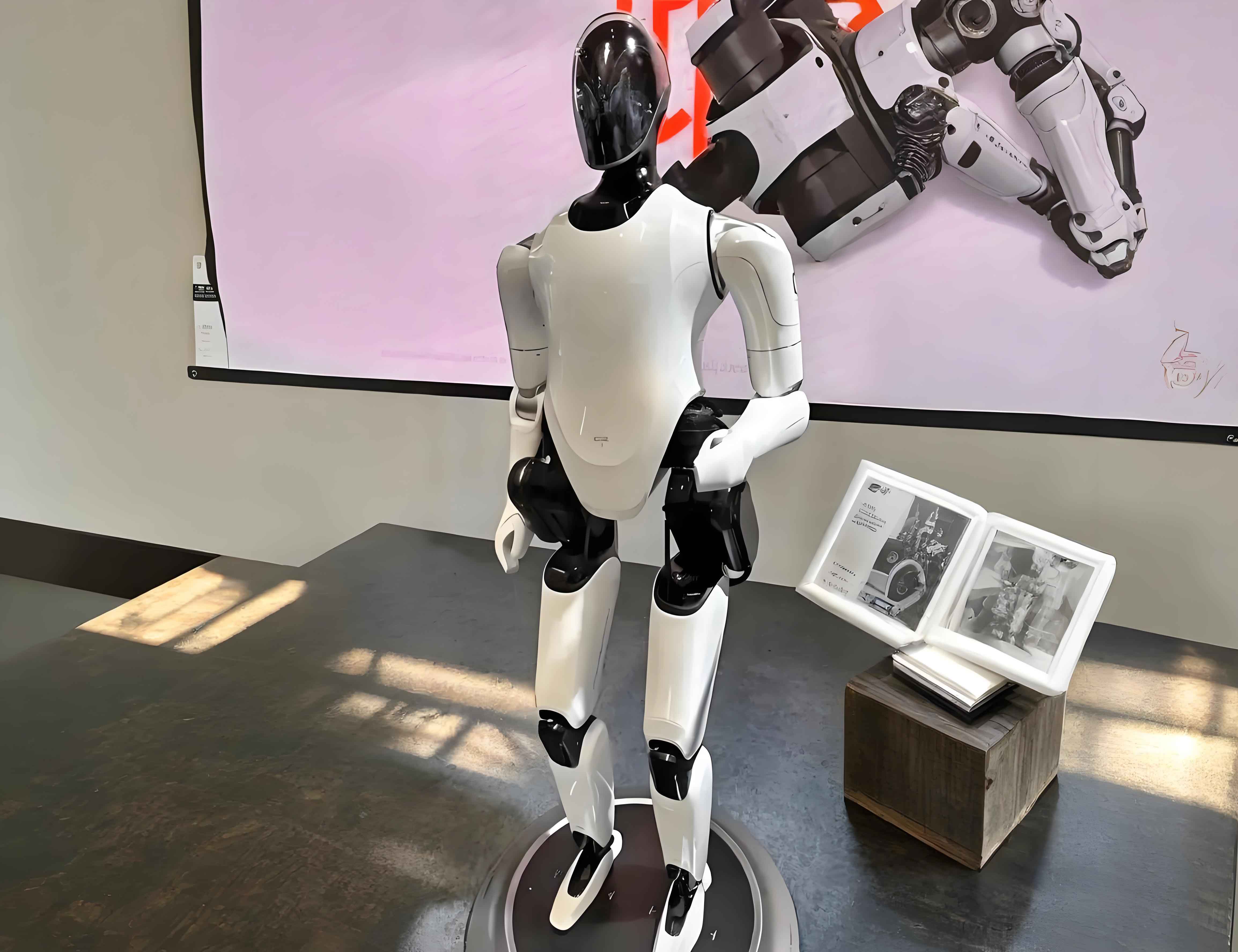
Embodied robots, particularly humanoid platforms, are rapidly moving from laboratory prototypes to real-world deployments in service, special operations, and complex unstructured environments. The joint actuator module, as the core execution unit of an embodied robot, directly determines the robot’s motion precision, dynamic response, and long-term operational reliability. Modern joint modules integrate a frameless torque motor, a precision reducer, an encoder, power electronics, and structural housing into a highly compact space. This high level of integration inevitably introduces coupled challenges in transmission accuracy, thermal management, and electromagnetic compatibility. In this study, I focus on the harmonic drive, which is the dominant reducer for mid-to-small joints of embodied robots, and propose a composite tooth profile design method. I then analyze the influence of key geometric parameters on contact stress and meshing performance via finite element simulations. A three-dimensional transmission performance model is established to investigate how the circular spline–flexspline interference affects backlash, lost motion, stiffness, and contact characteristics. Experimental tests are carried out to validate the trends predicted by the simulation. In parallel, I build a steady-state thermal model of the entire joint module to compare different housing heat dissipation structures, and I construct a three-dimensional electromagnetic model to evaluate the effect of a shielding layer on the magnetic field reaching the PCB and its copper loops. The results show that a carefully tuned interference between the circular spline and the flex spline can substantially improve transmission accuracy, while an oversized adjustment produces diminishing or even negative returns. The thermal simulations demonstrate that finned housing architectures effectively reduce the maximum temperature without adding active cooling components. Electromagnetic simulations reveal that although a shielding layer does not dramatically alter the overall magnetic field distribution on the PCB, it significantly attenuates the flux density at the chip location and the induced current density in critical PCB loops. These findings provide practical guidelines for the design and optimization of high-performance joint modules for embodied robots.
1. Introduction
The advancement of embodied robots demands joint actuators with ever-increasing power density and compactness. A typical joint module integrates a frameless torque motor, a harmonic reducer, a torque sensor, dual encoders, a motor driver, and a microcontroller unit (MCU) within an outer diameter of approximately 90 mm and an axial length of 80–100 mm. This spatial constraint creates three fundamental engineering problems. First, the harmonic reducer, which relies on the elastic deformation of a thin-walled flexspline, is highly sensitive to tooth geometry and assembly clearance. A poorly designed tooth profile or an inappropriate circular spline–flexspline interaction leads to uneven load sharing, elevated contact stress, and degraded positioning precision. Second, the frameless motor is embedded inside the structural housing with no dedicated cooling fan or liquid cooling channel. Copper and iron losses accumulate inside the module and raise its temperature, which in turn reduces motor efficiency, accelerates insulation aging, and may alter the harmonic drive’s meshing alignment due to thermal expansion. Third, the close physical proximity between the motor stator and the control PCB exposes sensitive components, such as the MCU and encoder interface chips, to time-varying magnetic fields. These fields can induce parasitic currents in PCB traces and cause signal integrity issues.
In this work, I address these three challenges in a systematic manner. I first propose a composite tooth profile design method for harmonic drives. The profile consists of an addendum transition arc, a convex arc, a tangent line segment, a concave arc, and a dedendum transition arc. This structure introduces smooth transitions at the tooth tip and root while preserving the essential geometry of conventional double-circular-arc teeth. I then perform two-dimensional contact simulations to study how the addendum coefficient, clearance coefficient, and pressure angle affect the maximum contact stress and pressure distribution. Based on these findings, I construct a full three-dimensional time-implicit finite element model of the harmonic drive to analyze the influence of the circular spline–flexspline adjustment on meshing clearance, contact area, the number of engaged tooth pairs, and equivalent torsional stiffness. Experiments on a dedicated test bench verify the simulation trends for lost motion, transmission error, and positioning accuracy.
For thermal management, I create a steady-state heat transfer model of the entire joint module. The motor rotor is represented as a constant-temperature heat source at 130 °C, and the ambient is set to 25 °C with natural convection. I compare four housing designs: a smooth housing (control), an axially slotted housing, a finned housing, and a housing with graphene patches. The results demonstrate that the finned design lowers the maximum steady-state temperature by approximately 9–10 °C compared with the control, while the other two strategies have a limited effect on the peak temperature.
For electromagnetic interference, I build a three-dimensional model of the motor–PCB assembly. I compare two configurations: one with a high-permeability shielding layer between the motor and the PCB and one without. The magnetic flux density at the motor, at the PCB region, and at the chip location, as well as the current density in the PCB loop, are extracted. Although the shielding layer has a negligible influence on the motor’s main magnetic path and the overall PCB field strength, it reduces the chip-level flux density by about 91% and the peak current density in the PCB loop by about 93%, confirming the benefit of localized magnetic shielding in a compact joint module.
This paper is organized as follows. Section 2 describes the composite tooth profile design and its contact mechanics analysis. Section 3 presents the three-dimensional transmission performance simulation and the experimental verification. Section 4 discusses the thermal and electromagnetic structure optimizations for the joint module. Section 5 summarizes the main conclusions and offers an outlook for future research.
2. Composite Tooth Profile Design for Harmonic Drives
2.1 Background and Rationale
Harmonic drives offer high reduction ratios, near-zero backlash, and compact construction, making them the preferred solution for the lower-torque, high-precision joints of embodied robots. However, the flexspline undergoes controlled periodic deformation every revolution, and its tooth profile must simultaneously satisfy conjugate meshing conditions, low contact stress, and high fatigue resistance. Traditional double-circular-arc profiles have sharp transitions at the tooth tip and root, which produce stress concentrations and excite high local contact pressure. To overcome this limitation, I design a composite multi-curve profile that incorporates transition arcs at the addendum and dedendum. The profile is parameterized so that each segment is smoothly connected with first-order continuity.
2.2 Mathematical Model of the Flexspline Tooth Profile
The tooth profile of the flexspline is constructed in a local coordinate system with the tooth symmetry axis as the reference. As shown in Figure 2.2 of the original reference, the profile comprises five regions: the addendum transition arc (EA), the convex arc (AB), the tangent line segment (BC), the concave arc (CD), and the dedendum transition arc (DF). Let \(s\) be the arc-length parameter along the profile. The parametric equations for each segment are expressed as follows.
For the addendum transition arc EA:
\[
\begin{cases}
x_{r0} = r_0 \cos\left(\frac{\pi}{2} – \frac{s}{r_0}\right) + x_{o0} \\[4pt]
y_{r0} = r_0 \sin\left(\frac{\pi}{2} – \frac{s}{r_0}\right) + y_{o0}
\end{cases}
\quad s \in (0, l_0)
\tag{2.1}
\]
For the convex arc AB:
\[
\begin{cases}
x_{r1} = r_1 \cos\left(\alpha – \frac{s}{r_1}\right) + x_{o1} \\[4pt]
y_{r1} = r_1 \sin\left(\alpha – \frac{s}{r_1}\right) + y_{o1}
\end{cases}
\quad s \in (l_0, l_1)
\tag{2.2}
\]
For the tangent line segment BC:
\[
\begin{cases}
x_{r2} = r_1 \cos\lambda + (s – l_1) \sin\lambda + x_{o1} \\[4pt]
y_{r2} = r_1 \sin\lambda – (s – l_1) \cos\lambda + y_{o1}
\end{cases}
\quad s \in (l_1, l_2)
\tag{2.3}
\]
For the concave arc CD:
\[
\begin{cases}
x_{r3} = -r_2 \cos\left(\lambda + \frac{s-l_2}{r_2}\right) + x_{o2} \\[4pt]
y_{r3} = -r_2 \sin\left(\lambda + \frac{s-l_2}{r_2}\right) + y_{o2}
\end{cases}
\quad s \in (l_2, l_3)
\tag{2.4}
\]
For the dedendum transition arc DF:
\[
\begin{cases}
x_{r4} = -r_3 \cos\left(\gamma + \frac{s-l_3}{r_3}\right) + x_{o3} \\[4pt]
y_{r4} = -r_3 \sin\left(\gamma + \frac{s-l_3}{r_3}\right) + y_{o3}
\end{cases}
\quad s \in (l_3, l_4)
\tag{2.5}
\]
Here, \(r_0, r_1, r_2, r_3\) are the radii of the transition/convex/concave arcs, \(\lambda\) is the tangent line inclination angle, \(\alpha\) is the pressure angle at the tooth tip, \(h_a\) and \(h_f\) are the addendum and dedendum heights, and \(e_0, e_1, e_2, e_3\) are the center offset distances of the respective arcs. The parameter definitions are summarized in Table 2.1.
| Parameter | Definition | Parameter | Definition |
|---|---|---|---|
| \(h_a\) | Addendum height | \(c_1\) | Convex arc center offset |
| \(h_f\) | Dedendum height | \(c_2\) | Concave arc center offset |
| \(r_0\) | Addendum transition radius | \(e_0\) | Addendum center distance |
| \(r_1\) | Convex arc radius | \(e_1\) | Convex center distance |
| \(r_2\) | Concave arc radius | \(e_2\) | Concave center distance |
| \(r_3\) | Dedendum transition radius | \(e_3\) | Dedendum center distance |
| \(L\) | Tangent line length | \(\lambda\) | Tangent line angle |
| \(d_h\) | Distance from root circle to neutral layer | \(\alpha\) | Pressure angle |
The baseline parameters of the flexspline used in this study correspond to a size-20 harmonic drive with a module of 0.273, a reduction ratio of 120, 240 flexspline teeth, and 242 circular spline teeth. Table 2.2 lists the detailed nominal values.
| Parameter | Value | Parameter | Value | Parameter | Value |
|---|---|---|---|---|---|
| \(h_a\) | 0.175 mm | \(r_3\) | 0.116 mm | \(e_0\) | 0.025 mm |
| \(h_f\) | 0.275 mm | \(L\) | 0.19 mm | \(e_1\) | 0.036 mm |
| \(r_0\) | 0.103 mm | \(d_h\) | 0.325 mm | \(e_2\) | 0.024 mm |
| \(r_1\) | 0.208 mm | \(c_1\) | 0.145 mm | \(e_3\) | 0.029 mm |
| \(r_2\) | 0.227 mm | \(c_2\) | 0.169 mm | \(\lambda\) | 12.6° |
2.3 Contact Mechanics Simulation
To quantify the influence of individual geometric parameters on the meshing performance of the harmonic drive, I adopt a controlled variable approach. Ten cases are designed by independently varying the addendum coefficient \(h_a^*\), the clearance coefficient \(c^*\), and the pressure angle \(\alpha\). The case matrix is presented in Table 2.3.
| Case | \(h_a^*\) | \(c^*\) | \(\alpha\) (°) | Purpose |
|---|---|---|---|---|
| 1 | 0.8 | 0.25 | 18 | Baseline |
| 2 | 0.6 | 0.25 | 18 | Vary \(h_a^*\) |
| 3 | 1.0 | 0.25 | 18 | Vary \(h_a^*\) |
| 4 | 1.2 | 0.25 | 18 | Vary \(h_a^*\) |
| 5 | 0.8 | 0.15 | 18 | Vary \(c^*\) |
| 6 | 0.8 | 0.35 | 18 | Vary \(c^*\) |
| 7 | 0.8 | 0.45 | 18 | Vary \(c^*\) |
| 8 | 0.8 | 0.25 | 20 | Vary \(\alpha\) |
| 9 | 0.8 | 0.25 | 22 | Vary \(\alpha\) |
| 10 | 0.8 | 0.25 | 25 | Vary \(\alpha\) |
Finite element simulations are conducted in Abaqus using a two-dimensional plane-strain approximation. The circular spline is modeled as a rigid body, the wave generator as a line rigid body, and the flexspline as a deformable body made of 40CrNiMoA steel. The material properties are listed in Table 2.4. The wave generator applies a rotation of 1 rpm in the second analysis step, and the output torque is ramped to 52 N·m. The maximum tooth contact stress and pressure distributions are evaluated.
| Material | Elastic modulus (GPa) | Poisson’s ratio | Density (kg/m\(^3\)) |
|---|---|---|---|
| 40CrNiMoA | 209 | 0.3 | 7850 |
2.3.1 Effect of Addendum Coefficient
Cases 1–4 compare the effect of \(h_a^* = 0.8, 0.6, 1.0, 1.2\). The maximum contact stresses are respectively 1642 MPa, 1445 MPa, 1738 MPa, and 2564 MPa. This trend shows that increasing the addendum coefficient enlarges the tooth height, raises the bending moment at the root, and intensifies the stress concentration at the tip. When \(h_a^*\) reaches 1.2, the maximum contact stress is 56% higher than the baseline, indicating that a large addendum coefficient is detrimental to the load-carrying capacity of the flexspline. Table 2.5 summarizes the results.
| Case | \(h_a^*\) | Maximum contact stress (MPa) | Relative change |
|---|---|---|---|
| 2 | 0.6 | 1445 | −12.0% |
| 1 | 0.8 | 1642 | — |
| 3 | 1.0 | 1738 | +5.8% |
| 4 | 1.2 | 2564 | +56.2% |
2.3.2 Effect of Clearance Coefficient
Cases 1, 5, 6, and 7 use \(c^* = 0.25, 0.15, 0.35, 0.45\), resulting in maximum contact stresses of 1642 MPa, 1102 MPa, 2646 MPa, and 1273 MPa, respectively. The response is non-monotonic. A smaller clearance coefficient reduces the root gap and allows a more favorable contact pattern, whereas \(c^* = 0.35\) produces the worst stress concentration. Further increasing \(c^*\) to 0.45 surprisingly reduces the stress again, indicating a complex interaction between the root fillet shape and the loading path. Table 2.6 lists the results.
| Case | \(c^*\) | Maximum contact stress (MPa) | Relative change |
|---|---|---|---|
| 5 | 0.15 | 1102 | −32.9% |
| 1 | 0.25 | 1642 | — |
| 6 | 0.35 | 2646 | +61.1% |
| 7 | 0.45 | 1273 | −22.5% |
2.3.3 Effect of Pressure Angle
Cases 1, 8, 9, and 10 employ \(\alpha = 18°, 20°, 22°, 25°\), giving maximum contact stresses of 1642 MPa, 1179 MPa, 1037 MPa, and 1468 MPa, respectively. The stress first decreases with increasing pressure angle, reaches a minimum at \(\alpha = 22°\), and then increases again. This behavior indicates that a moderate pressure angle improves the load distribution along the tooth flank, but an excessively large pressure angle changes the direction of the resultant force and degrades the local contact condition. Table 2.7 summarizes the results.
| Case | \(\alpha\) (°) | Maximum contact stress (MPa) | Relative change |
|---|---|---|---|
| 1 | 18 | 1642 | — |
| 8 | 20 | 1179 | −28.2% |
| 9 | 22 | 1037 | −36.8% |
| 10 | 25 | 1468 | −10.6% |
The contact mechanics analysis demonstrates that the composite tooth profile enables independent control over key design parameters. The optimal design should balance the addendum coefficient, clearance coefficient, and pressure angle according to the specific load spectrum of the embodied robot joint. In particular, the pressure angle around \(22°\) gives the most uniform pressure distribution, which is beneficial for reducing wear and extending fatigue life.
3. Three-Dimensional Transmission Performance Simulation
3.1 Geometric Mapping of the Circular Spline Tooth Profile
The flexspline tooth profile alone does not determine the transmission performance; the conjugate circular spline profile must be generated from the flexspline motion. I employ a geometric mapping method to obtain the theoretical circular spline tooth profile. The flexspline tooth profile is expressed in its own coordinate system \(S_1\). A point \(p_1 = (x_1, y_1)\) on the flexspline tooth is transformed into the circular spline coordinate system \(S_2\) via a homogeneous transformation matrix \(M_{21}\):
\[
\begin{bmatrix} x_2 \\ y_2 \\ 1 \end{bmatrix}
=
M_{21}
\begin{bmatrix} x_1 \\ y_1 \\ 1 \end{bmatrix}
\tag{3.1}
\]
The matrix \(M_{21}\) accounts for the rotation and elastic deformation of the flexspline:
\[
M_{21} =
\begin{bmatrix}
\cos\xi & \sin\xi & \rho \sin\varepsilon \\
-\sin\xi & \cos\xi & \rho \cos\varepsilon \\
0 & 0 & 1
\end{bmatrix}
\tag{3.2}
\]
where \(\xi = \varepsilon + \mu\), \(\varepsilon\) is the relative rotation angle of the deformed flexspline end, \(\mu\) is the additional normal rotation, and \(\rho\) is the radial deformation parameter. The conjugate condition for the envelope is
\[
\frac{\partial x_2(s,\theta)}{\partial s} \frac{\partial y_2(s,\theta)}{\partial \theta}
=
\frac{\partial x_2(s,\theta)}{\partial \theta} \frac{\partial y_2(s,\theta)}{\partial s}
\tag{3.3}
\]
Solving (3.3) together with the coordinate transformation yields the theoretical circular spline tooth profile. This method provides a rigorous analytical link between the flexspline geometry, the deformation kinematics, and the resulting circular spline shape. The generated profile is then used as the geometric basis for the three-dimensional finite element model.
3.2 Three-Dimensional Finite Element Model
I build a complete three-dimensional model of the harmonic drive in SolidWorks, including the circular spline, flexspline, wave generator cam, and flexspline bearing. To reduce the computational cost, the cam and the bearing inner race are merged into a single equivalent elliptical cam, and the bearing balls and rings are merged into a simplified flexible bearing. The final model is imported into Abaqus, where the circular spline and the cam are treated as discrete rigid bodies, while the flexspline and the flexible bearing are deformable bodies. Table 3.1 lists the mesh statistics.
| Component | Element count (million) | Element type |
|---|---|---|
| Flexspline | 1.26 | C3D8R |
| Circular spline | 0.14 | R3D4 |
| Cam | 0.047 | R3D4 |
| Flexible bearing | 0.23 | C3D8R |
| Total | 1.677 | — |
The static analysis consists of two steps. In the first step, the cam expands the flexspline and establishes the initial contact with the circular spline. In the second step, an output torque of 52 N·m is applied in the positive direction, then unloaded, then applied in the negative direction, and finally unloaded again. This loading sequence provides the hysteresis loop necessary for computing lost motion and backlash. The friction coefficient at the tooth meshing interface is set to 0.3, while the contact between the bearing outer ring and the flexspline inner surface is assumed to be perfectly rough.
3.3 Influence of Circular Spline–Flexspline Adjustment
To study the effect of the mesh clearance between the circular spline and the flexspline, I systematically enlarge the circular spline tooth thickness relative to the nominal envelope, which effectively reduces the clearance. Six configurations are analyzed: the unadjusted case and cases with adjustments of 2.5 μm, 5 μm, 7.5 μm, 10 μm, and 12.5 μm. The contact clearance contours show that as the interference increases, the low-clearance region along the major axis expands. The contact stress distribution becomes more uniform, and the number of simultaneously engaged tooth pairs increases. Table 3.2 lists the number of engaged tooth pairs at several time instants for each adjustment.
| Adjustment (μm) | 0% torque (0 s) | +52 N·m (0.1 s) | 0% torque (0.2 s) | −52 N·m (0.3 s) | 0% torque (0.4 s) |
|---|---|---|---|---|---|
| 0 | 43 | 56 | 44 | 55 | 44 |
| 2.5 | 45 | 56 | 45 | 56 | 45 |
| 5 | 45 | 56 | 46 | 56 | 46 |
| 7.5 | 47 | 54 | 46 | 55 | 46 |
| 10 | 47 | 55 | 46 | 55 | 46 |
| 12.5 | 47 | 56 | 47 | 55 | 47 |
The proportion of engaged tooth pairs increases from approximately 36% in the unadjusted case to over 39% in the 12.5 μm case. The contact area grows correspondingly, as shown by the time-averaged values in Table 3.3. A larger contact area reduces the average contact pressure and improves the load-sharing capability.
| Adjustment (μm) | Contact area (mm\(^2\)) | Average contact pressure (MPa) | Peak contact stress (MPa) |
|---|---|---|---|
| 0 | 4.91 | 10.6 | 1637 |
| 2.5 | 5.12 | 10.2 | 1589 |
| 5 | 5.36 | 9.7 | 1512 |
| 7.5 | 5.68 | 9.2 | 1418 |
| 10 | 6.02 | 8.7 | 1335 |
| 12.5 | 6.41 | 8.1 | 1256 |
The hysteresis curves are post-processed to extract the lost motion and backlash. Table 3.4 reports the results for all adjustment levels. A monotonic decreasing trend is observed: the lost motion drops from 64.23 arcsec to 3.45 arcsec as the adjustment increases from 0 to 12.5 μm, and the backlash drops from 43.14 arcsec to 1.98 arcsec. The equivalent torsional stiffness simultaneously rises, with the high-load stiffness \(K_3\) experiencing the most pronounced increase.
| Adjustment (μm) | Lost motion (arcsec) | Backlash (arcsec) | \(K_1\) (N·m/rad) | \(K_2\) (N·m/rad) | \(K_3\) (N·m/rad) |
|---|---|---|---|---|---|
| 0 | 64.23 | 43.14 | 25800 | 41400 | 51200 |
| 2.5 | 55.18 | 35.70 | 28600 | 44300 | 54800 |
| 5 | 43.66 | 27.85 | 32100 | 48200 | 60500 |
| 7.5 | 23.42 | 13.90 | 38900 | 55100 | 68400 |
| 10 | 8.21 | 5.02 | 46700 | 62300 | 82100 |
| 12.5 | 3.45 | 1.98 | 56200 | 71800 | 96300 |
These results clearly indicate that a moderate reduction of the circular spline–flexspline clearance is beneficial for the transmission accuracy and stiffness of the harmonic drive. However, the improvement is not perfectly linear. The difference between the 10 μm and 12.5 μm cases is smaller than the difference between the 5 μm and 7.5 μm cases, suggesting that the optimal adjustment region may depend on the elastic deformation of the flexspline and the available assembly tolerances. Excessive interference could induce unwanted preload and increase wear. Therefore, the appropriate adjustment must be selected based on the specific application requirements of the embodied robot joint.
3.4 Influence of Wave Generator Profile
The wave generator cam shape determines the deformation pattern of the flexspline. In this study, I use a composite-profile cam consisting of a parabolic segment near the major axis, a transition arc, and a side arc. The cam profile is shown schematically in the original reference, and its quarter geometry is controlled by the parabolic end angle \(A\). I keep the major axis, the parabolic coefficient \(K\), and the transition radius \(R\) constant, and I vary \(A\) among 15°, 25°, 30°, and 35°. Table 3.5 lists the four cam cases.
| Case | Major axis (mm) | Parabolic coefficient \(K\) | Transition radius \(R\) (mm) | Parabolic end angle \(A\) (°) |
|---|---|---|---|---|
| 1 | 36.1684 | −0.029 | 7 | 15 |
| 2 | 36.1684 | −0.029 | 7 | 25 |
| 3 | 36.1684 | −0.029 | 7 | 30 |
| 4 | 36.1684 | −0.029 | 7 | 35 |
Simulation results show that as \(A\) increases, the cam profile transitions more smoothly from the major axis to the side region. Consequently, the flexspline deformation becomes more gradual and the tooth meshing proceeds with a more uniform clearance distribution. The contact stress concentration near the major axis is alleviated, and the proportion of engaged teeth rises. Table 3.6 summarizes the lost motion, backlash, and stiffness values for the four cam profiles. The optimal performance is observed for Case 4 with \(A = 35°\), which produces the smallest lost motion of 4.47 arcsec and the smallest backlash of 2.60 arcsec, while the high-load stiffness \(K_3\) reaches 143,210 N·m/rad.
| Case | Lost motion (arcsec) | Backlash (arcsec) | \(K_1\) (N·m/rad) | \(K_2\) (N·m/rad) | \(K_3\) (N·m/rad) |
|---|---|---|---|---|---|
| 1 (15°) | 18.04 | 11.50 | 33717 | 51667 | 56050 |
| 2 (25°) | 8.23 | 5.02 | 56671 | 62821 | 87094 |
| 3 (30°) | 6.01 | 3.25 | 72184 | 75650 | 89467 |
| 4 (35°) | 4.47 | 2.60 | 89610 | 89689 | 143210 |
Furthermore, the finite element results reveal that the number of engaged tooth pairs increases from about 41 pairs for Case 1 to about 51 pairs for Case 4 at rated torque. This confirms that the wave generator profile is an equally important design variable for improving the load-sharing behavior of the harmonic drive.
3.5 Experimental Verification
To validate the simulation trends, I perform experiments on a comprehensive test bench for harmonic reducers. The test bench measures lost motion, transmission error, absolute positioning accuracy, and repeatability under different circular spline adjustment conditions. The wave generator with the optimal profile from Case 4 is used in all experimental trials. The circular spline is adjusted to four different interference levels: 5 μm, 7.5 μm, 10 μm, and 12.5 μm. Table 3.7 lists the measured precision indicators.
| Adjustment (μm) | Lost motion | Forward transmission error | Reverse transmission error | Total transmission error | Positioning accuracy | Repeatability |
|---|---|---|---|---|---|---|
| 5 | 60 | 94 | 92 | 101 | 98 | 67 |
| 7.5 | 11 | 35 | 35 | 37 | 40 | 32 |
| 10 | 15 | 52 | 55 | 54 | 38 | 32 |
| 12.5 | 5 | 52 | 53 | 52 | 30 | 17 |
The experimental data show that the lost motion decreases dramatically when the adjustment is increased from 5 μm to 7.5 μm and then remains low at 12.5 μm. The positioning accuracy and repeatability also improve with larger adjustments, although the 10 μm case has a slightly higher transmission error than the 7.5 μm case. This non-monotonic behavior is consistent with the simulation prediction that a moderate interference improves the meshing condition, but an excessive adjustment could introduce additional elastic deformation or misalignment that partially counteracts the benefit. Overall, the experimental results confirm the practical effectiveness of optimizing the circular spline–flexspline matching relationship for high-precision joint drives of embodied robots.
4. Thermal and Electromagnetic Structure Optimization for the Joint Module
4.1 Thermal Structure Optimization
The joint module of an embodied robot operates under high current density and frequent dynamic load changes. In the absence of active cooling, the heat generated in the stator windings and the iron core accumulates inside the housing. The temperature rise not only reduces motor efficiency and demagnetizes the permanent magnets, but also degrades the grease in the harmonic reducer and shifts the dimensions of the structural components. I therefore construct a steady-state thermal model of the entire joint module to compare the cooling effects of alternative housing designs.
The three-dimensional geometry includes the motor stator, rotor, harmonic reducer, bearings, and the aluminum housing. The motor rotor is set to a constant temperature of 130 °C as the thermal source. The ambient temperature is 25 °C, and the external convective heat transfer coefficient is set to 10 W/(m\(^2\)·K), which represents natural convection in still air. The contact thermal conductance between adjacent parts is set to 80 W/(m\(^2\)·K). Table 4.1 lists the thermal conductivity values used in the model.
| Component | Material | Thermal conductivity (W/(m·K)) |
|---|---|---|
| Housing | Aluminum alloy | 167 |
| Stator core | Silicon steel | 22 |
| Rotor magnet | NdFeB | 20 |
| Harmonic drive | Alloy steel 40Cr | 45 |
| Bearing | Bearing steel | 46 |
| PCB | FR-4 | 0.3 |
Four housing designs are compared: (a) a smooth housing as the control, (b) an axially slotted housing, (c) a finned housing, and (d) a housing with graphene patches attached to the outer surface. The steady-state temperature distributions are computed in Abaqus using the steady-state heat transfer module. Table 4.2 summarizes the maximum and minimum temperatures obtained for each design.
| Housing design | Maximum temperature (°C) | Minimum temperature (°C) |
|---|---|---|
| Control (smooth) | 127.1 | 24.94 |
| Axially slotted | 127.1 | 25.00 |
| Finned | 117.4 | 25.00 |
| Graphene-patched | 127.1 | 24.74 |
It is evident that the finned housing reduces the maximum temperature by roughly 9.7 °C compared with the control, while the other designs do not change the peak temperature significantly. The finned structure increases the effective heat transfer surface area, thereby enhancing natural convection without consuming additional power or increasing the module volume. The axially slotted housing produces a slightly more uniform surface temperature but fails to reduce the core temperature because the increase in surface area is insufficient. The graphene patches improve the in-plane thermal spreading on the housing surface but do not alter the dominant resistance of external natural convection. Therefore, the finned housing is the most effective passive thermal solution for a joint module of an embodied robot.
4.2 Electromagnetic Interference Simulation and Shielding Optimization
In the highly integrated joint module, the frameless motor is located in close proximity to the PCB that carries the MCU, gate drivers, and communication circuits. The time-varying magnetic field generated by the motor can leak into the PCB area and induce interference. To evaluate the potential electromagnetic interference, I build a three-dimensional electromagnetic model of the motor–PCB assembly in COMSOL Multiphysics. Two configurations are considered: one with a shielding layer between the motor and the PCB, and one without. The shielding layer is modeled as a high-permeability material with a relative permeability of 2000 and a very low electrical conductivity of \(10^{-6}\) S/m, which represents a magnetic shielding material rather than a conductive metal plate.
The simplified PCB model includes the board substrate, a simple copper loop that represents a critical signal or power trace, and a region designated as the MCU chip location. The motor is modeled with a permanent magnet rotor, a stator core, and copper windings. The material definitions are provided in Table 4.3. The magnet is N52 grade sintered NdFeB, the stator and rotor cores are soft iron, and the surrounding domain is air. The excitation is set to a typical operating condition for the frameless motor.
| Component | Material | Role |
|---|---|---|
| Air domain | Air | Propagation medium |
| Winding | Copper | Conductive current path |
| Core | Soft iron (without losses) | Main magnetic path |
| Permanent magnet | N52 (sintered NdFeB) | Magnetic field source |
| PCB | FR-4 equivalent | Substrate for copper loop and chip |
After meshing with local refinement at the air gap, the permanent magnet, and the PCB, I extract four indicators: the motor magnetic flux density, the PCB region magnetic flux density, the magnetic flux density at the chip location, and the induced current density in the PCB loop. Table 4.4 compares the maximum values for the shielded and unshielded configurations.
| Indicator | With shielding layer | Without shielding layer | Relative change |
|---|---|---|---|
| Motor \(|B|_{max}\) (T) | 6.61 | 6.58 | +0.46% |
| PCB region \(|B|_{max}\) (mT) | 41.3 | 40.4 | +2.23% |
| Chip location \(|B|_{max}\) (mT) | 3.14 | 34.9 | −91.0% |
| PCB loop current density \(|J|_{max}\) (A/m\(^2\)) | 1.08×10\(^{-4}\) | 1.64×10\(^{-5}\) | −93.4% |
| Induced loop voltage (mV) | 3.49×10\(^{-4}\) | 3.32×10\(^{-4}\) | +5.12% |
Several observations can be made from these results. First, the shielding layer has a negligible effect on the motor’s internal magnetic field, with the peak flux density changing by only 0.46%. This is expected because the shield is placed outside the main magnetic circuit. Second, the overall magnetic field amplitude on the PCB region is not significantly reduced; in fact, the peak value increases by 2.23%. This indicates that the shield redistributes the magnetic flux rather than uniformly absorbing it. Third, the chip location experiences a dramatic reduction of 91.0% in the peak flux density, from 34.9 mT to 3.14 mT. This is a highly beneficial effect because the MCU and other sensitive components are more vulnerable to local magnetic fields than the average PCB field. Fourth, the peak current density in the PCB copper loop is reduced by 93.4%, confirming that the shield suppresses the induced eddy-like currents in the loop. However, the overall induced loop voltage remains nearly unchanged, which implies that the dominant coupling pathway might not be through the loop area but rather through direct field leakage to specific segments. Despite this, the substantial reduction at the chip location and the loop’s local current density demonstrates that a well-designed magnetic shield can effectively mitigate electromagnetic interference in critical regions of the joint module.
The spatial distribution plots further support these quantitative conclusions. In the unshielded case, the chip location shows large areas of orange and red, indicating magnetic flux densities above 30 mT. When the shielding layer is inserted, the chip region becomes predominantly blue and light green, corresponding to flux densities below 5 mT. The PCB loop current density also evolves from a concentrated high-value pattern at the corners and long edges to a more uniform and lower-amplitude distribution. These results confirm the following design insight for the joint module of an embodied robot: if the main concern is the average magnetic field over the entire PCB, a simple high-permeability shield may not offer much benefit. However, if the concern is the adverse effect on specific control chips and critical loops, the shield provides a substantial improvement and is a worthwhile structural optimization.
5. Conclusion and Outlook
In this study, I have systematically investigated the harmonic drive design and the thermal-electromagnetic structure optimization of a joint actuator module for embodied robots. The main contributions and conclusions are summarized as follows.
(1) A composite multi-curve tooth profile for the harmonic drive is proposed. The profile consists of a tip transition arc, a convex arc, a tangent segment, a concave arc, and a dedendum transition arc. The parametric model allows independent adjustment of the addendum coefficient, the clearance coefficient, and the pressure angle. Finite element contact simulations show that the addendum coefficient has a strong influence on contact stress; a large addendum coefficient significantly increases stress concentration. The clearance coefficient exhibits a non-monotonic influence, and the pressure angle has an optimal value around 22° that minimizes the maximum contact stress. This design method provides a practical way to tailor the tooth profile to the load requirements of an embodied robot joint.
(2) A three-dimensional transmission performance model of the harmonic drive is established using a geometric mapping method to generate the conjugate circular spline profile. The simulation results reveal that incrementally increasing the circular spline–flexspline interference reduces the lost motion and backlash while increasing the equivalent torsional stiffness. The contact area and the number of engaged tooth pairs also increase, leading to more uniform load sharing. Experimental tests confirm the overall trend, but also reveal that the improvement saturates or slightly deteriorates beyond a certain adjustment. Therefore, an optimal interference range must be selected based on the elastic deformation capacity and practical assembly tolerances.
(3) The wave generator cam profile has a significant impact on the transmission performance. A composite cam with a larger parabolic end angle produces a smoother deformation transition in the flexspline, which improves the meshing clearance distribution, reduces contact stress, increases the number of engaged teeth, and lowers the lost motion and backlash. The optimal cam profile in the studied range corresponds to a parabolic end angle of 35°.
(4) In terms of thermal management, steady-state simulations of the joint module show that a finned housing can reduce the maximum temperature by about 9.7 °C compared with a smooth housing under natural convection. Axially slotted housings and graphene patches have a much smaller effect on the peak temperature, but the graphene patch can improve the surface temperature uniformity. The finned housing is recommended as an effective passive cooling solution for high-power-density joint modules.
(5) In terms of electromagnetic compatibility, a high-permeability shielding layer placed between the motor and the PCB does not alter the motor’s internal magnetic flux density nor the overall PCB field strength significantly. However, it reduces the peak magnetic flux density at the chip location by about 91% and the peak current density in the PCB loop by about 93%. This demonstrates that the shield is highly effective in suppressing electromagnetic interference in localized sensitive zones, which is critical for the stable operation of the MCU and encoder interfaces in a compact joint module.
Future work will extend the static electromagnetic analysis to dynamic operating conditions, including PWM switching effects and the coupling with control signal integrity. Furthermore, the thermal model can be refined with experimentally derived loss maps and transient heat loading. The coupling between thermal expansion and harmonic drive accuracy will also be investigated to obtain a more complete multi-physics design methodology for the joint modules of embodied robots.