
I designed and developed an experimental teaching platform and an associated teaching method for the motion control system of an industrial robot end-effector. The central motivation for this work is that modern intelligent manufacturing requires an industrial robot to do far more than repeat a taught path. In contact-rich operations such as grinding, polishing, deburring, and precision assembly, the industrial robot end-effector is the component that directly interacts with the workpiece, and its control performance often determines final surface quality, dimensional accuracy, and process stability. Therefore, I structured the teaching content around a concrete engineering scenario: constant-force grinding performed by an industrial robot. In this scenario, the industrial robot must move along a planned trajectory while the end-effector maintains a stable contact force against a workpiece whose geometry and local stiffness may vary.
The experimental platform I developed integrates a six-degree-of-freedom serial industrial robot, a 2R1T force-controlled end-effector, a real-time industrial controller, servo drives, incremental encoders, and a six-axis force sensor. The software environment is built on a real-time automation framework, and the overall system contains four functional modules: motion control, logic operation control, adaptive constant-force variable-admittance control, and human-machine interaction. With this platform, I propose a progressive experimental teaching method that leads students from single-axis point-to-point motion control, to multi-axis coordinated trajectory interpolation, and finally to force-position hybrid control for constant-force grinding. The method is intended to help students understand not only how an industrial robot moves, but also how an industrial robot regulates physical interaction with its environment.
In the following sections, I present the design rationale, the hardware and software architecture, the mathematical models used in teaching, the detailed experimental procedures, representative results, and the assessment strategy. I use tables and formulas throughout to summarize the essential relationships and performance indicators. The discussion is written from my perspective as the designer and instructor of the experimental teaching system.
The first design principle I adopted is that the teaching platform must expose the complete control chain of an industrial robot end-effector rather than hiding it behind a black-box interface. Students should be able to see how a desired motion command becomes a servo drive signal, how encoder feedback closes the position loop, how a force sensor closes the force loop, and how an adaptive controller modifies motion commands in real time. The second principle is modularity. Each hardware component and software module can be tested independently before being integrated into the full industrial robot grinding task. The third principle is measurability. Every experiment must produce quantitative data, including position error, velocity smoothness, force error, and force fluctuation, so that students can evaluate and improve controller performance.
I begin with the experimental platform. The physical system includes a wrist-offset six-degree-of-freedom serial industrial robot, a 2R1T end-effector driven by three voice coil motors, an industrial PC, servo drives, incremental encoders, a six-axis force sensor, and an air pump for the machining tool. The serial industrial robot provides gross positioning and orientation. The 2R1T end-effector provides fine motion and force regulation. The industrial PC communicates with the servo drives and the force sensor through a real-time Ethernet fieldbus. The servo drives power the voice coil motors and implement the inner current, velocity, and position loops. The incremental encoders measure the voice coil motor positions. The six-axis force sensor measures the contact force between the tool and the workpiece. The air pump drives the pneumatic machining tool. This combination allows the industrial robot end-effector to perform precise motion control and stable constant-force control during grinding.
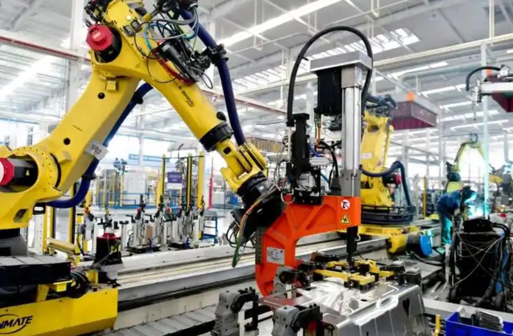
The hardware architecture is summarized in Table 1. I use this table in the teaching material to show students how each component contributes to the overall industrial robot end-effector control system. The table also clarifies which signals are command signals, which are feedback signals, and which are power or pneumatic signals.
| Component | Main function | Signal type | Role in the industrial robot end-effector system |
|---|---|---|---|
| Six-degree-of-freedom serial industrial robot | Gross positioning and orientation | Motion command and joint feedback | Carries the end-effector to the vicinity of the workpiece |
| 2R1T end-effector | Fine motion and force control | Position and force commands | Provides two rotational and one translational degree of freedom for contact control |
| Voice coil motors | High-bandwidth linear actuation | Current and position | Generate fast displacement for force regulation |
| Industrial PC | Real-time computation and communication | Fieldbus and control signals | Runs the control modules and coordinates all devices |
| Servo drives | Motor power amplification and closed-loop control | Current, velocity, position | Drive the voice coil motors and enforce inner loops |
| Incremental encoders | Position measurement | Digital pulse feedback | Provide position feedback for the voice coil motors |
| Six-axis force sensor | Contact force measurement | Analog or digital force feedback | Provides the force signal for constant-force control |
| Air pump | Tool actuation | Pneumatic | Drives the grinding or machining tool |
The software architecture is equally important. I developed the control system in a real-time automation environment. The software contains four functional modules: motion control, logic operation control, adaptive constant-force variable-admittance control, and human-machine interaction. The motion control module generates position, velocity, and trajectory commands. The logic operation control module manages enable signals, mode switching, safety interlocks, and state transitions. The adaptive constant-force variable-admittance control module adjusts the motion command according to the force error. The human-machine interaction module displays position, velocity, force, and system status in real time, and it allows students to set parameters and start or stop experiments. Table 2 lists these modules and their teaching functions.
| Software module | Core function | Key variables | Teaching purpose |
|---|---|---|---|
| Motion control module | Generate single-axis and multi-axis motion commands | Position, velocity, acceleration, interpolation time | Teach point-to-point and trajectory motion |
| Logic operation control module | Manage modes, enable signals, and safety logic | State flags, error codes, interlocks | Teach system integration and fault handling |
| Adaptive constant-force variable-admittance control module | Regulate contact force through force feedback | Force error, admittance parameters, neural network weights | Teach force-position hybrid control |
| Human-machine interaction module | Visualize data and accept user commands | Position, velocity, force, status, parameters | Teach experiment operation and data interpretation |
The control flow of the industrial robot end-effector system follows a clear sequence. First, the student sets the desired parameters through the human-machine interface. Second, the motion control module generates the corresponding motion command. Third, the logic operation control module receives and transfers the command to the numerical control module. Fourth, the numerical control module interprets the command and sends it to the virtual axes, which then drive the servo drives and voice coil motors. Fifth, when the end-effector contacts the workpiece, the six-axis force sensor collects the contact force and feeds it back to the adaptive constant-force variable-admittance control module. Sixth, the module adjusts the motion command according to the force deviation, thereby achieving constant-force control. This closed-loop chain is the technical foundation of the industrial robot grinding experiment, and it is also the central teaching thread that connects all experimental steps.
To make the control principles precise, I introduce several mathematical models in the teaching material. The first is the single-axis motion error. For a desired position $$p_d(t)$$ and an actual position $$p_a(t)$$, the instantaneous position error is
$$ e_p(t) = p_d(t) – p_a(t). $$
The maximum absolute error and the root-mean-square error over a time interval are respectively
$$ e_{\max} = \max_{1 \le k \le N} \left| p_d(k) – p_a(k) \right|, $$
$$ \mathrm{RMSE} = \sqrt{ \frac{1}{N} \sum_{k=1}^{N} \left( p_d(k) – p_a(k) \right)^2 }. $$
These two indicators are used in the single-axis experiment to compare jog motion, relative motion, and absolute motion. The velocity smoothness can be evaluated by the standard deviation of the velocity signal or by the maximum jerk:
$$ j_{\max} = \max_{1 \le k \le N-2} \left| \frac{v(k+2) – 2v(k+1) + v(k)}{\Delta t^2} \right|. $$
For multi-axis coordinated motion, I teach students to describe the trajectory as a parametric curve. For a straight-line segment from point $$p_0$$ to point $$p_1$$, the position command is
$$ p(t) = p_0 + (p_1 – p_0) \frac{t}{T}, \quad 0 \le t \le T, $$
where $$T$$ is the total interpolation time. The velocity vector is
$$ v(t) = \frac{p_1 – p_0}{T}. $$
If the three axes must arrive synchronously, the interpolation must satisfy
$$ \frac{v_i}{L_i} = \text{constant}, \quad i = 1,2,3, $$
where $$v_i$$ is the velocity of axis $$i$$ and $$L_i$$ is the displacement of axis $$i$$. This equation explains why the control system automatically distributes different velocities to different axes while keeping the same arrival time.
The most important model for the advanced experiment is the admittance control model. In general, an admittance controller relates the external force to a position correction through a virtual mass-damper-spring system:
$$ M_d \ddot{x} + B_d \dot{x} + K_d x = F_{ext} – F_d, $$
where $$M_d$$ is the virtual inertia, $$B_d$$ is the virtual damping, $$K_d$$ is the virtual stiffness, $$x$$ is the position correction, $$F_{ext}$$ is the external contact force, and $$F_d$$ is the desired force. In the Laplace domain, the transfer function from force error to position correction is
$$ \frac{X(s)}{F_{ext}(s) – F_d(s)} = \frac{1}{M_d s^2 + B_d s + K_d}. $$
When the virtual stiffness is set to zero, the controller behaves as a pure force regulator and allows the end-effector to comply with the workpiece surface. When the virtual stiffness is increased, the controller becomes stiffer and tracks position more strongly, but it may also produce larger force oscillations. This trade-off is one of the key concepts I want students to understand through experiments.
For comparison, I also teach a classical PID-optimized admittance controller. The outer-loop force controller can be written as
$$ u(t) = K_p e_f(t) + K_i \int_0^t e_f(\tau) d\tau + K_d \frac{d e_f(t)}{dt}, $$
where
$$ e_f(t) = F_d – F_m(t), $$
and $$F_m(t)$$ is the measured force. The PID controller is simple and intuitive, but its fixed gains make it less effective when the contact environment changes during grinding. To overcome this limitation, I introduce a neural-network adaptive constant-force variable-admittance controller. The core idea is to use a radial basis function neural network to compensate for uncertainties and to adjust the admittance parameters online.
The radial basis function network used in the experiment has an input vector $$x$$, a hidden layer with $$n$$ neurons, and an output. The Gaussian basis function of the $$j$$-th hidden neuron is
$$ h_j(x) = \exp\left( -\frac{\| x – c_j \|^2}{2 \sigma_j^2} \right), \quad j = 1,2,\dots,n, $$
where $$c_j$$ is the center and $$\sigma_j$$ is the width. The network output is
$$ y = \sum_{j=1}^{n} w_j h_j(x), $$
where $$w_j$$ is the weight of the $$j$$-th neuron. In the teaching experiment, the network output is used to compensate the force error and to adjust the admittance parameters. The loss function can be defined as
$$ E = \frac{1}{2} c_1 e_f^2 + \frac{1}{2} c_2 \dot{e}_f^2, $$
where $$c_1$$ and $$c_2$$ are gain coefficients. The weight update law includes a learning term and a momentum term:
$$ \Delta w_j = \eta e_f h_j(x), $$
$$ \dot{w}_j = -\eta \frac{\partial E}{\partial w_j} + \alpha \Delta w_j, $$
where $$\eta$$ is the learning factor and $$\alpha$$ is the momentum factor. These equations give students a concrete view of how an adaptive controller can improve force tracking without a precise analytical model of the workpiece.
Once the platform and models are introduced, I organize the experimental teaching into three progressive experiments and one evaluation stage. The first experiment is single-axis motion control. The second experiment is multi-axis coordinated motion control. The third experiment is constant-force grinding control. The final stage is experimental evaluation and improvement. Table 3 summarizes the overall teaching sequence and the expected learning outcomes.
| Stage | Experiment | Core task | Expected outcome |
|---|---|---|---|
| 1 | Single-axis motion control | Jog, relative, and absolute motion of one voice coil motor | Understand point-to-point positioning and error evaluation |
| 2 | Multi-axis coordinated motion control | Linear interpolation with three axes in one channel | Understand trajectory planning and synchronization |
| 3 | Constant-force grinding control | Force-position hybrid control with a desired force of 15 N | Understand admittance control and adaptive force regulation |
| 4 | Evaluation and improvement | Analyze data, tune parameters, and compare controllers | Develop engineering debugging and optimization skills |
Before any experiment begins, I require students to perform a complete equipment check. They verify that the incremental encoder position display is normal, that the air pump for the end-effector is operating correctly, and that the end-effector is at the origin position. They then connect the control host to the industrial PC through a network cable and activate the real-time environment. They use a scope-view tool to monitor motion parameters during the machining process. This preparation step is essential because an industrial robot end-effector system can produce unsafe motion if the axes are not enabled correctly or if the force sensor is not calibrated.
For the single-axis motion control experiment, I ask students to map the virtual axes in the software to the physical axes obtained from the input/output scan. This mapping establishes a real-time data channel between the computed command and the physical industrial robot end-effector. The students then complete homing, axis selection, and speed setting in manual mode. They execute three motion modes: jog motion, relative motion, and absolute motion. In each mode, they read the position and velocity from the axis status window and check the status lamp and error code for abnormalities. The tool speed is set to 3000 r/min, and the single-axis speed is set to 1.0 mm/s. Table 4 shows the single-axis motion sequence used in the experiment.
| Step | Motion mode | Command | Purpose |
|---|---|---|---|
| 1 | Jog | Move axis 8 by 6.0 mm | Test manual continuous motion and basic response |
| 2 | Relative | Move axis 8 by -8.0 mm, then by 5.0 mm | Test incremental positioning |
| 3 | Absolute | Move axis 8 to -5.4 mm, then to -2.0 mm, then relative by -7.0 mm | Test absolute positioning and mixed commands |
The experimental results show that all three motion modes can move the voice coil motor smoothly to the target position. Compared with jog motion, relative motion and absolute motion reduce the maximum position error by 0.024 mm and 0.044 mm, respectively. They also reduce the root-mean-square error by 0.040 mm and 0.056 mm, respectively. These results are summarized in Table 5. I use this table to help students see that the choice of motion mode is not merely a matter of convenience; it directly affects positioning accuracy and repeatability. The single-axis experiment therefore establishes the precision positioning foundation for the later constant-force grinding experiment.
| Motion mode | Maximum position error reduction relative to jog (mm) | RMSE reduction relative to jog (mm) | Observed behavior |
|---|---|---|---|
| Jog | 0.000 | 0.000 | Smooth but less precise for final positioning |
| Relative | 0.024 | 0.040 | Better incremental accuracy |
| Absolute | 0.044 | 0.056 | Best final positioning accuracy among the three modes |
In the multi-axis coordinated motion control experiment, students switch to automatic mode and enter the multi-axis control interface. They enable the axes and set the initial positions of the three virtual axes to
$$ P_0 = (6, 3, 5) \ \text{mm}, $$
with an initial speed of 10 mm/min. The first trajectory starts at
$$ P_1 = (-2, 2, 1) \ \text{mm} $$
and ends at
$$ P_2 = (4, 8, -5) \ \text{mm}. $$
After the first segment, the speed is set to 15 mm/min. The second trajectory starts at
$$ P_2 = (4, 8, -5) \ \text{mm} $$
and ends at
$$ P_3 = (2, 6, 3) \ \text{mm}. $$
The three axes are then combined into the same numerical control interpolation channel. When the combination indicator is on, the student presses start, and the system executes the planned trajectory while the interface updates the position and velocity of each axis in real time. Table 6 lists the trajectory parameters used in the experiment.
| Segment | Start point (mm) | End point (mm) | Speed (mm/min) | Interpolation type |
|---|---|---|---|---|
| Initial | (6, 3, 5) | — | 10 | — |
| Segment 1 | (-2, 2, 1) | (4, 8, -5) | 10 | Linear |
| Segment 2 | (4, 8, -5) | (2, 6, 3) | 15 | Linear |
The results show that the motion control system automatically calculates and distributes the required speed for each axis according to the length of the planned trajectory, so that all axes reach the specified position synchronously. At trajectory switching points and speed step changes, no obvious oscillation appears, which indicates good dynamic stability. The multi-axis coordinated motion experiment provides the trajectory foundation for the constant-force control experiment. It allows the industrial robot end-effector to move smoothly along a prescribed path during grinding, which is necessary for precise force-position hybrid control and stable constant-force output.
I evaluate the multi-axis experiment using three indicators: synchronization error, trajectory tracking error, and velocity smoothness. The synchronization error between axis $$i$$ and axis $$j$$ can be defined as
$$ e_{ij}(t) = \frac{p_i(t)}{L_i} – \frac{p_j(t)}{L_j}, $$
where $$L_i$$ and $$L_j$$ are the total displacements of the two axes. Ideally, this error should remain close to zero for linear interpolation. The trajectory tracking error is computed from the difference between the commanded path and the actual path. The velocity smoothness is evaluated from the standard deviation of the velocity signal. Table 7 summarizes the qualitative and quantitative observations from the multi-axis experiment.
| Indicator | Definition | Observed result | Teaching interpretation |
|---|---|---|---|
| Synchronization error | Normalized difference between axis positions | Small and bounded | Axes arrive together |
| Trajectory tracking error | Deviation from the planned line | Within acceptable range | Interpolation is accurate |
| Velocity smoothness | Variation of velocity during motion | No obvious oscillation | System is dynamically stable |
The third and most important experiment is constant-force grinding control. The task is to make the industrial robot end-effector contact the workpiece and maintain a desired grinding force of 15 N while the industrial robot moves along a planned trajectory. The six-degree-of-freedom industrial robot provides gross position control. The 2R1T end-effector provides fine motion and force control. The six-axis force sensor measures the contact force. The adaptive constant-force variable-admittance controller adjusts the motion command according to the force error. I introduce two controllers for comparison: a PID-optimized admittance controller and a neural-network adaptive constant-force variable-admittance controller. The first represents a classical fixed-model approach. The second represents an intelligent approach that can adjust parameters online and compensate for uncertainties and environmental changes.
The parameter sets used in the constant-force experiment are listed in Table 8. I explain to students that these parameters are not arbitrary; they determine the bandwidth, stability, and steady-state accuracy of the force loop. The inner loop PID parameters are tuned first because the voice coil motor must track the position command quickly and accurately. The outer force loop parameters are then tuned to achieve the desired force response without excessive overshoot or oscillation.
| Parameter | Value | Controller | Effect |
|---|---|---|---|
| Motor speed | 3000 r/min | Tool | Sets the grinding speed |
| Inner loop proportional gain $$K_p$$ | 24 | PID | Improves position response |
| Inner loop integral gain $$K_i$$ | 30 | PID | Reduces steady-state error |
| Inner loop derivative gain $$K_d$$ | 1.5 | PID | Damps oscillations |
| Hidden neurons $$n$$ | 32 | RBF network | Approximation capacity |
| Learning factor $$\eta$$ | 0.0001 | RBF network | Adaptation speed |
| Loss gain $$c_1$$ | 0.8 | RBF network | Force error weighting |
| Loss gain $$c_2$$ | 0.012 | RBF network | Force derivative weighting |
| Momentum factor $$\alpha$$ | 0.002 | RBF network | Weight update smoothing |
| Gaussian width $$\sigma$$ | 0.2 | RBF network | Basis function width |
| Initial inertia $$M_d$$ | 1 | Admittance | Virtual mass |
| Initial damping $$B_d$$ | 15 | Admittance | Virtual damping |
| Initial stiffness $$K_d$$ | 0 | Admittance | Compliance behavior |
| Outer loop proportional gain $$K_p$$ | 18 | PID optimized admittance | Force response |
| Outer loop integral gain $$K_i$$ | 25 | PID optimized admittance | Force steady-state error |
| Outer loop derivative gain $$K_d$$ | 1.2 | PID optimized admittance | Force damping |
| Sampling period | 2 ms | Force loop | Real-time force data acquisition |
The experimental procedure for constant-force grinding is as follows. First, the student confirms that the industrial robot end-effector is at a safe starting position. Second, the student sets the desired force to 15 N in the human-machine interface. Third, the industrial robot moves the end-effector toward the workpiece. Fourth, when contact is detected by the six-axis force sensor, the adaptive constant-force variable-admittance control module is activated. Fifth, the controller adjusts the motion command according to the force error. Sixth, the student records the force data, position data, and controller parameters. Seventh, the student compares the performance of the two controllers. Table 9 lists the experimental steps and the corresponding observations.
| Step | Action | Observation | Control focus |
|---|---|---|---|
| 1 | Set desired force to 15 N | Target force displayed | Reference input |
| 2 | Move industrial robot toward workpiece | Force begins to rise | Approach phase |
| 3 | Detect contact | Force sensor signal increases | Contact transition |
| 4 | Activate adaptive controller | Force error is computed | Force loop activation |
| 5 | Adjust motion command | End-effector compliance changes | Force-position hybrid control |
| 6 | Record data | Force, position, and time data saved | Performance evaluation |
| 7 | Compare controllers | Different force fluctuations | Controller assessment |
Representative results show that the neural-network adaptive constant-force variable-admittance controller has a slight overshoot at the beginning, but it quickly adjusts itself. During the approach and maintenance of the 15 N target force, it exhibits stronger adaptability and disturbance rejection than the PID-optimized admittance controller. It can adjust control parameters online according to the real-time force error, so the system enters and remains in a stable state quickly. The average force error is 0.16 N, and the steady-state fluctuation range is within ±1.5 N. In contrast, the PID-optimized admittance controller responds quickly in the initial stage, but during continuous grinding it shows larger force fluctuations. Its average force error is 0.31 N, and its steady-state fluctuation range is ±3.2 N. Table 10 summarizes the performance comparison.
| Controller | Average force error (N) | Steady-state fluctuation (N) | Dynamic behavior | Disturbance rejection |
|---|---|---|---|---|
| Neural-network adaptive constant-force variable-admittance | 0.16 | ±1.5 | Fast adaptation after slight overshoot | Strong |
| PID-optimized admittance | 0.31 | ±3.2 | Fast initial response but larger steady-state oscillation | Moderate |
To quantify the force tracking performance, I define the average absolute force error as
$$ \bar{e}_F = \frac{1}{N} \sum_{k=1}^{N} \left| F_d – F_m(k) \right|, $$
and the force fluctuation as
$$ \Delta F = \max_{1 \le k \le N} F_m(k) – \min_{1 \le k \le N} F_m(k). $$
These definitions are used in the data analysis stage. Students also compute the standard deviation of the force signal:
$$ \sigma_F = \sqrt{ \frac{1}{N} \sum_{k=1}^{N} \left( F_m(k) – \bar{F}_m \right)^2 }, $$
where $$\bar{F}_m$$ is the mean measured force. The smaller the values of $$\bar{e}_F$$, $$\Delta F$$, and $$\sigma_F$$, the better the constant-force control performance. This quantitative approach helps students move from qualitative observation to engineering evaluation.
The experimental teaching method also includes a systematic evaluation and improvement stage. Students are asked to adjust motion parameters to optimize trajectory performance and to tune neural-network learning factors, loss function gains, and admittance parameters to improve force control accuracy and robustness. I encourage them to follow a structured debugging cycle: set initial parameters, run the experiment, collect data, analyze the error, identify the dominant cause, adjust one parameter group at a time, and repeat. Table 11 presents the debugging cycle and the associated engineering skills.
| Debugging step | Action | Data used | Skill developed |
|---|---|---|---|
| 1 | Set initial parameters | Parameter table | System configuration |
| 2 | Run the industrial robot experiment | Motion and force data | Experimental operation |
| 3 | Collect and visualize data | Scope view records | Data acquisition |
| 4 | Analyze error and fluctuation | RMSE, average error, standard deviation | Quantitative analysis |
| 5 | Identify dominant cause | Trajectory, force, and timing signals | Fault diagnosis |
| 6 | Adjust one parameter group | Controller gains and network weights | Parameter tuning |
| 7 | Repeat and compare | Performance tables | Iterative optimization |
I also include a fault-handling table in the teaching material because real industrial robot end-effector experiments often involve communication errors, axis enable failures, force sensor drift, or unexpected contact. Table 12 lists common issues and remedies. This table helps students develop safe and efficient troubleshooting habits.
| Issue | Possible cause | Remedy | Safety note |
|---|---|---|---|
| Axis does not enable | Drive not powered, interlock active, or mapping error | Check power, interlocks, and virtual-physical axis mapping | Keep emergency stop accessible |
| No force feedback | Sensor cable disconnected or calibration lost | Check cable, recalibrate sensor, and verify signal range | Do not command contact without force feedback |
| Large force oscillation | Admittance damping too low or PID gains too high | Increase damping or reduce proportional gain | Move end-effector away from workpiece before tuning |
| Position drift | Encoder issue or mechanical looseness | Check encoder, homing, and mechanical connections | Re-home before restarting |
| Communication timeout | Network disturbance or incorrect fieldbus configuration | Check cable, cycle power, and verify configuration | Stop all motion before resetting |
From a pedagogical perspective, the three experiments form a complete skill chain. The single-axis experiment teaches precise positioning. The multi-axis experiment teaches trajectory coordination. The constant-force experiment teaches force-position hybrid control. Together, they allow students to understand the full motion control system of an industrial robot end-effector. I emphasize that the industrial robot itself is not merely a positioner in this context; it is part of a larger controlled interaction system. The industrial robot end-effector is the component that transforms a motion command into a controlled physical interaction, and the force sensor closes the loop that makes constant-force grinding possible.
I also use the platform to discuss the difference between position control and force control. In pure position control, the objective is to minimize
$$ e_p(t) = p_d(t) – p_a(t). $$
In pure force control, the objective is to minimize
$$ e_f(t) = F_d – F_m(t). $$
In force-position hybrid control, the objective is to regulate both the motion and the contact force. A common formulation is
$$ \min \left( \alpha \| e_p \|^2 + \beta \| e_f \|^2 \right), $$
where $$\alpha$$ and $$\beta$$ are weighting factors. This formulation helps students understand that industrial robot grinding is a multi-objective control problem. The end-effector must follow the surface geometry while maintaining a stable force. If the force is too high, the workpiece may be damaged. If the force is too low, the surface may be poorly finished. The adaptive controller adjusts the balance between position tracking and force tracking in real time.
The platform also supports discussion of stability. For the admittance controller, the closed-loop stability depends on the virtual mass, damping, stiffness, and the environment stiffness. A simplified interaction model can be written as
$$ F_{ext} = K_e (x_a – x_w), $$
where $$K_e$$ is the workpiece stiffness, $$x_a$$ is the actual end-effector position, and $$x_w$$ is the workpiece surface position. Combining this with the admittance model gives a coupled system whose stability can be analyzed by root locus or Nyquist methods. I do not require students to perform full stability proofs in the introductory experiment, but I introduce the concept so that they understand why parameter tuning matters. The neural-network adaptive controller can adjust the admittance parameters online, which can improve robustness when $$K_e$$ varies along the workpiece.
In terms of experimental data analysis, I ask students to produce the following quantitative summaries:
1. Position accuracy: maximum error and RMSE for jog, relative, and absolute motion.
2. Velocity smoothness: standard deviation of velocity and maximum jerk for single-axis motion.
3. Multi-axis synchronization: normalized synchronization error and trajectory tracking error.
4. Force tracking: average absolute force error, standard deviation, and steady-state fluctuation range.
5. Controller comparison: a table of performance indicators for the PID-optimized admittance controller and the neural-network adaptive controller.
These summaries are not merely reporting tasks. They require students to connect control theory with measured behavior. For example, a large force fluctuation may indicate insufficient damping, a high learning rate, or a mismatch between the admittance model and the actual workpiece stiffness. A large position error may indicate an incorrect motion mode, a servo tuning issue, or a mechanical backlash problem. By linking symptoms to causes, students develop diagnostic reasoning.
I also include an assessment rubric that evaluates both technical and professional skills. Table 13 shows the rubric. The rubric is designed to reward safe operation, accurate data analysis, correct use of formulas, and thoughtful improvement. It also encourages students to reflect on the limitations of each controller.
| Assessment area | Indicator | Weight | Expected evidence |
|---|---|---|---|
| Safety and preparation | Equipment check and safe operation | 15% | Checklist and no unsafe actions |
| Single-axis control | Correct mode selection and error analysis | 15% | Position and RMSE tables |
| Multi-axis control | Trajectory setup and synchronization evaluation | 20% | Trajectory data and synchronization error |
| Constant-force control | Force tracking and controller comparison | 30% | Force curves and performance table |
| Improvement and reflection | Parameter tuning and engineering reasoning | 20% | Debugging log and revised results |
The experimental results confirm that the platform has good motion control and constant-force control performance. The single-axis experiment achieves smooth positioning with reduced error in relative and absolute modes. The multi-axis experiment achieves synchronous trajectory motion without obvious oscillation. The constant-force experiment achieves a stable 15 N grinding force, with the neural-network adaptive controller outperforming the PID-optimized admittance controller in steady-state force accuracy and disturbance rejection. These outcomes demonstrate that the proposed teaching method is effective and that the platform provides a realistic environment for learning industrial robot end-effector control technology.
I also believe that the teaching method can be extended in several ways. One extension is to introduce different workpiece materials and surface geometries. Another is to add vision feedback so that the industrial robot end-effector can adjust to surface features in real time. A third is to implement a digital twin of the industrial robot end-effector system, allowing students to test controller parameters in simulation before running the physical experiment. A fourth is to introduce multi-sensor fusion, combining force, vision, and position data for more robust grinding control. These extensions would further strengthen the connection between intelligent manufacturing theory and industrial robot practice.
In summary, I designed an experimental platform and a progressive teaching method for the motion control system of an industrial robot end-effector. The platform integrates a six-degree-of-freedom serial industrial robot, a 2R1T end-effector, real-time control hardware, servo drives, encoders, and a six-axis force sensor. The software includes motion control, logic control, adaptive constant-force variable-admittance control, and human-machine interaction modules. The teaching method guides students from single-axis positioning to multi-axis trajectory coordination and finally to constant-force grinding. Through formula-based analysis, table-based comparison, and hands-on debugging, students learn how an industrial robot end-effector regulates both motion and force. The experimental results show that the platform can achieve precise motion control and stable constant-force control, and that the neural-network adaptive controller provides better force tracking and robustness than the classical PID-optimized admittance controller. I conclude that the proposed platform and method offer a practical and effective way to teach industrial robot end-effector motion control and to prepare students for advanced work in intelligent manufacturing.