
I present a systematic modal analysis method for industrial robots that combines a multi-posture model with the poly-reference least squares complex frequency-domain method, abbreviated as pLSCF. The motivation for this work is the observation that industrial robots exhibit strongly posture-dependent dynamic behavior and pronounced multi-joint coupling. Their low-order modes shift with joint configuration, and reliable identification of these modes is essential for accuracy, stability, and reliability in tasks such as assembly, handling, machining, and welding. In this study I establish two boundary postures for a six-degree-of-freedom industrial robot, perform hammer and shaker modal tests, and identify the first three modal parameters using pLSCF. The results show that the first natural frequency decreases by 8.68% from one boundary posture to the other, while the second and third natural frequencies increase by 21.23% and 17.90%, respectively. The damping ratios of both configurations remain within 0.968%–1.745%. The modal assurance criterion values confirm good spatial independence, with all off-diagonal values below 0.06 for the first configuration and a maximum of 0.18 for the first–second mode pair in the second configuration. These findings provide a reliable basis for dynamic modeling, posture-dependent stability assessment, and structural optimization of industrial robots.
1. Introduction
Industrial robots are central to modern intelligent manufacturing. They are widely deployed in assembly, pick-and-place, milling, drilling, welding, and inspection. In all these applications, the dynamic characteristics of the complete machine significantly affect operational accuracy, motion stability, and system reliability. Natural frequencies, damping ratios, and dynamic stiffness determine how force, torque, and inertia influence the motion performance of components and of the complete industrial robot. Because industrial robots typically contain multiple joints and complex coupling paths, they are prone to vibration during high-speed motion or under varying payloads. Therefore, understanding their vibration behavior is of great importance.
Modal analysis is a fundamental method for studying structural dynamic characteristics. By extracting modal frequencies, mode shapes, and damping parameters, modal analysis can effectively describe the dynamic behavior of a system under external loads. For industrial robots, modal analysis supports structural design optimization, vibration suppression, and joint performance enhancement. Compared with a single structural component, an industrial robot with multiple joints and coupled links exhibits obvious multi-order modal characteristics. These modal characteristics can be used to predict dynamic behavior under different postures, including dynamic stiffness and joint performance. Modal testing usually begins with simulation analysis to determine the target frequency band and dominant mode shapes. Then, experimental modal analysis is performed using either hammer excitation or shaker excitation. For industrial robots, modal analysis often starts from individual components such as joints, links, and reducers, and then extends to the complete machine.
However, the modal characteristics of industrial robots are strongly posture-dependent. Earlier studies have examined how frequency response functions vary along an end-effector path. Other studies have measured natural frequencies for several joint rotation angles. The influence of configuration on structural modes has also been reported. Nevertheless, existing research often focuses on frequency variation under a limited number of postures. Stable identification of weak responses and adjacent modes under multi-joint coupling conditions remains insufficient. Modal parameters must be extracted accurately from frequency response functions. Although line–angle compound vibration measurement can be accurate, it is often complex. In this work I use acceleration sensors for single-direction vibration measurement because they are convenient and practical. Single-degree-of-freedom methods and the least squares complex frequency-domain method are mainly based on a single reference frequency response. The single-degree-of-freedom method is suitable for structures with well-separated modes and weak coupling. The least squares complex frequency-domain method can identify dense modes through stabilization diagrams, but it is sensitive to local signal-to-noise ratio and sensor placement. The pLSCF method is a multi-reference frequency-domain least squares method based on multi-degree-of-freedom concepts. For multi-configuration testing of industrial robots, moving hammer excitation uses multi-excitation-point joint fitting, so strong response information compensates for weak response modes and reduces identification bias caused by channel noise and local nonlinearity. Single-point fixed excitation constructs multiple response channels, so strong response channels compensate for weak response channels and reduce identification bias caused by local noise and joint nonlinearity. Therefore, pLSCF is suitable for modal identification of multi-joint coupled industrial robots. I therefore propose a modal analysis method based on a multi-posture model and pLSCF. First, I establish and simplify a multi-posture model based on stiffness boundary configurations. Then, I perform modal tests on the two models using hammer and shaker methods. Finally, I extract modal information using pLSCF and analyze, verify, and discuss the results with mode shapes and modal assurance criteria.
2. pLSCF Algorithm for Industrial Robots
Because industrial robots have multiple degrees of freedom, strong coupling, and configuration-dependent behavior, modal parameters under different postures can differ significantly. The pLSCF method can fully use multi-reference excitation information and achieve stable identification of modal parameters under multiple postures of industrial robots. The algorithm consists of two main parts. First, basic parameters such as modal frequency, damping ratio, and participation vectors are estimated. Second, the mode shapes are estimated using the pLSCF formulation.
2.1 Basic Parameter Estimation
Let \(N_o\), \(N_i\), and \(N_f\) denote the number of outputs, inputs, and spectral lines, respectively. The output index is \(o=1,2,\ldots,N_o\), and the spectral line index is \(f=1,2,\ldots,N_f\). Based on a right matrix fraction description, the frequency response function matrix \(\mathbf{H} \in \mathbb{C}^{N_o \times N_i}\) is modeled as
$$ \mathbf{H}(\Omega_f) = \mathbf{B}(\Omega_f)\mathbf{A}^{-1}(\Omega_f), $$
where
$$ \mathbf{B}(\Omega_f)=\sum_{j=0}^{n}\boldsymbol{\beta}_j \Omega_f^j,\qquad \mathbf{A}(\Omega_f)=\sum_{j=0}^{n}\boldsymbol{\alpha}_j \Omega_f^j. $$
Here, \(\boldsymbol{\beta}_j \in \mathbb{C}^{N_o \times N_i}\) and \(\boldsymbol{\alpha}_j \in \mathbb{C}^{N_i \times N_i}\) are the numerator and denominator polynomial coefficient matrices, respectively. The two polynomials usually have the same order \(n\), but different orders can be selected if necessary. Because the polynomial coefficients are considered in the real domain, an \(n\)-th order polynomial can identify at most \(n/2\) modes.
The polynomial coefficients are computed from the error equation
$$ \mathbf{e}_{o,f}=w_{o,f}\left(\sum_{j=0}^{n}\boldsymbol{\beta}_{o,j}\Omega_f^j-\mathbf{H}_{o,f}\sum_{j=0}^{n}\boldsymbol{\alpha}_{j}\Omega_f^j\right), $$
where \(\mathbf{H}_{o,f}\) is the measured frequency response function, \(\mathbf{e}_{o,f} \in \mathbb{C}^{N_i}\) is the residual, and \(w_{o,f} \in \mathbb{C}\) is an optional weighting coefficient. The weighting coefficient can be chosen according to the uncertainty of the frequency response function. A least squares cost function is then constructed as
$$ \ell=\sum_{o=1}^{N_o}\sum_{f=1}^{N_f}\mathrm{tr}\left(\mathbf{e}_{o,f}^{H}\mathbf{e}_{o,f}\right), $$
where \((\cdot)^{H}\) denotes the complex conjugate transpose. By solving this least squares problem and partitioning the coefficients into numerator and denominator blocks, I obtain the normalized denominator polynomial coefficients. Then a companion matrix is constructed, and its eigenvalue decomposition yields the discrete-time poles. The highest-order denominator coefficient is normalized to the identity matrix:
$$ \boldsymbol{\alpha}_n=\mathbf{I}. $$
The companion matrix can be written as
$$ \mathbf{D}_c= \begin{bmatrix} -\boldsymbol{\alpha}_1 & -\boldsymbol{\alpha}_2 & \cdots & -\boldsymbol{\alpha}_{n-1} & -\boldsymbol{\alpha}_n \\ \mathbf{I} & \mathbf{0} & \cdots & \mathbf{0} & \mathbf{0} \\ \mathbf{0} & \mathbf{I} & \cdots & \mathbf{0} & \mathbf{0} \\ \vdots & \vdots & \ddots & \vdots & \vdots \\ \mathbf{0} & \mathbf{0} & \cdots & \mathbf{I} & \mathbf{0} \end{bmatrix}. $$
The matrices \(\mathbf{x}\) and \(\mathbf{y}\) contain the right and left eigenvectors, respectively, of all considered modes. The diagonal matrix
$$ \mathbf{Z}=\mathrm{diag}(z_1,\ldots,z_{N_m}) $$
contains the discrete-time poles, and \(N_m\) is the total number of identified modes. These discrete-time poles are converted into continuous-time poles using
$$ \lambda_r=\frac{\ln(z_r)}{T_s}. $$
Therefore, the damped natural frequency \(f_{d,r}\) and damping ratio \(\xi_r\) can be obtained as
$$ f_{d,r}=\frac{|\lambda_r|}{2\pi},\qquad \xi_r=-\frac{\mathrm{Re}(\lambda_r)}{|\lambda_r|}. $$
The participation vector \(\mathbf{L}_r \in \mathbb{C}^{N_i}\) can be obtained from the left eigenvector \(\mathbf{y}\) of the companion matrix \(\mathbf{D}_c\). The \(r\)-th column of \(\mathbf{y}\) can be expressed as
$$ \mathbf{y}_r= \begin{bmatrix} z_r^{n-1}\mathbf{L}_r^{T} & \cdots & z_r\mathbf{L}_r^{T} & \mathbf{L}_r^{T} \end{bmatrix}^{T}. $$
Therefore, by taking the last \(N_i\) rows of \(\mathbf{y}\) and normalizing each column with respect to its maximum element, I obtain the normalized participation vector matrix \(\widetilde{\mathbf{L}} \in \mathbb{C}^{N_i \times N_m}\), which is used in the next subsection to estimate the mode shapes.
The identified discrete-time poles depend on the model order, and physical poles appear as complex conjugate pairs with positive damping ratios. I use a threefold stability criterion based on natural frequency, damping ratio, and mode shape. The initial criteria are: relative error of natural frequency less than 1%, relative error of damping ratio less than 5%, and modal assurance criterion for the corresponding mode shape not less than 0.9. According to the frequency response function data quality, I tightened the actual screening thresholds to 0.8%, 4%, and 0.95. The stabilization diagram is used to determine the model order and extract modal parameters. Table 1 summarizes the stabilization criteria.
| Parameter | Initial criterion | Tightened criterion used here |
|---|---|---|
| Natural frequency relative error | <1% | <0.8% |
| Damping ratio relative error | <5% | <4% |
| Mode shape MAC | \(\geq 0.9\) | \(\geq 0.95\) |
2.2 Mode Shape Estimation
The continuous-time poles \(\lambda_r\) and normalized participation vectors \(\widetilde{\mathbf{L}}_r\) obtained in the previous subsection are used here to estimate the mode shapes \(\boldsymbol{\phi}_r\) for \(r=1,2,\ldots,N_m\). The lower residual \(\boldsymbol{\rho}_l\) and upper residual \(\boldsymbol{\rho}_u\) are used to compensate for modes outside the considered frequency band. For an acceleration frequency response function, the upper residual term is \(\omega_f^2\boldsymbol{\rho}_u\), while for a displacement frequency response function the lower residual is \(\boldsymbol{\rho}_l/\omega_f^2\). Taking acceleration frequency response functions as an example,
$$ \mathbf{H}(\omega_f)=\sum_{r=1}^{N_m}\left(\frac{\boldsymbol{\phi}_r\mathbf{L}_r^{T}}{j\omega_f-\lambda_r}+\frac{\boldsymbol{\phi}_r^{*}\mathbf{L}_r^{H}}{j\omega_f-\lambda_r^{*}}\right)+\boldsymbol{\rho}_l+\omega_f^2\boldsymbol{\rho}_u. $$
Here, the frequency response function matrix \(\mathbf{H} \in \mathbb{C}^{N_o \times N_i}\) is obtained by stacking \(\mathbf{H}_{o,f}\) for \(o=1,\ldots,N_o\). The symbol \((\cdot)^{*}\) denotes complex conjugation. The lower residual term \(\boldsymbol{\rho}_l\) represents the approximately constant contribution of the analysis band to the acceleration frequency response function. The upper residual term \(\omega_f^2\boldsymbol{\rho}_u\) represents the equivalent influence of truncated modes above the band. In this equation, the mode shapes and residual terms are the only unknowns and are solved using least squares.
Taking the conjugate transpose of the above equation and introducing the diagonal matrices
$$ \mathbf{D}_f=\mathrm{diag}\left(\frac{1}{j\omega_f-\lambda_1},\ldots,\frac{1}{j\omega_f-\lambda_{N_m}}\right), $$
$$ \mathbf{D}_f^{*}=\mathrm{diag}\left(\frac{1}{j\omega_f-\lambda_1^{*}},\ldots,\frac{1}{j\omega_f-\lambda_{N_m}^{*}}\right), $$
the frequency response function model can be rearranged into a linear form. The normalized participation vector matrix \(\widetilde{\mathbf{L}}\) and the mode shape matrix \(\boldsymbol{\Phi}\) are arranged as
$$ \widetilde{\mathbf{L}}=\begin{bmatrix}\widetilde{\mathbf{L}}_1 & \cdots & \widetilde{\mathbf{L}}_{N_m}\end{bmatrix},\qquad \boldsymbol{\Phi}=\begin{bmatrix}\boldsymbol{\phi}_1 & \cdots & \boldsymbol{\phi}_{N_m}\end{bmatrix}. $$
To convert the frequency response function matrix into a unified linear equation, I introduce vectorization and the Kronecker product identity:
$$ \mathrm{vec}\left(\widetilde{\mathbf{L}}\mathbf{D}_f\boldsymbol{\Phi}^{T}\right)=\left(\mathbf{I}\otimes\widetilde{\mathbf{L}}\mathbf{D}_f\right)\mathrm{vec}\left(\boldsymbol{\Phi}\right). $$
Here, \(\mathrm{vec}(\cdot)\) denotes column-wise stacking of matrix elements, and \(\otimes\) denotes the Kronecker product. The overdetermined linear system is obtained by stacking the real and imaginary parts of the frequency response function at all frequency points:
$$ \mathbf{h}=\mathbf{A}\mathbf{X}. $$
Here, \(\mathbf{h}\) is the observation vector formed by stacking the real and imaginary parts of the frequency response function at all frequency points, \(\mathbf{A}\) is the coefficient matrix, and \(\mathbf{X}\) is the unknown parameter vector. The variables satisfy
$$ \mathbf{h}=\begin{bmatrix}\mathbf{h}_1 & \cdots & \mathbf{h}_{N_f}\end{bmatrix}^{T},\qquad \mathbf{A}=\begin{bmatrix}\mathbf{A}_1 & \cdots & \mathbf{A}_{N_f}\end{bmatrix}^{T}. $$
The number of frequency lines selected in the test satisfies \(2N_f \geq 2N_mN_i + 4N_i\), and the coefficient matrix \(\mathbf{A}\) has full column rank, so the least squares parameters are identifiable. Here, \(N_i\) is the number of reference points, \(N_f\) is the number of frequency lines, and \(N_m\) is the model order. Thus, the number of spectral lines is sufficiently large. The solution is
$$ \mathbf{X}=\mathbf{A}^{\dagger}\mathbf{h}, $$
where \((\cdot)^{\dagger}\) denotes the Moore–Penrose pseudoinverse. Because the participation vectors have already been normalized and the residual terms \(\boldsymbol{\phi}_r^{T}\widetilde{\mathbf{L}}_r\) are uniquely determined, the mode shapes are also uniquely determined.
3. Multi-Posture Model of Industrial Robots
3.1 Model Establishment
The test object is a six-degree-of-freedom industrial robot with a payload of 70 kg, a reach of 2100 mm, and a repeat positioning accuracy of \(\pm 0.05\) mm. Its complete structure consists of a base, shoulder, large arm, elbow, small arm, wrist, and end-effector connection. The components rotate about joint axes, so the robot can achieve different working postures. The base is fixed to a laboratory concrete floor through a steel mounting plate. The robot is connected using eight M20×60 bolts, tightened in stages according to the specified preload torque.
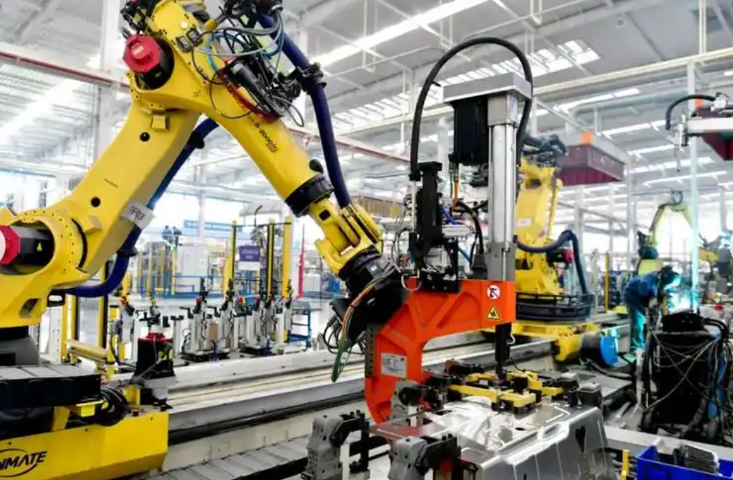
The six-degree-of-freedom industrial robot has a typical multi-rigid-body serial structure, and its dynamic characteristics are closely related to joint configuration. For a given joint configuration \(\mathbf{q}=\begin{bmatrix}q_1 & \cdots & q_6\end{bmatrix}^{T}\), the vibration equation of the robot can be written as
$$ \mathbf{M}(\mathbf{q})\ddot{\mathbf{x}}+\mathbf{C}(\mathbf{q})\dot{\mathbf{x}}+\mathbf{K}(\mathbf{q})\mathbf{x}=\mathbf{0}, $$
where \(q_i\) is the rotation angle of the \(i\)-th joint, \(\mathbf{M}(\mathbf{q})\) is the mass matrix, \(\mathbf{C}(\mathbf{q})\) is the damping matrix, and \(\mathbf{K}(\mathbf{q})\) is the stiffness matrix. Neglecting damping, the modal equation corresponding to the \(i\)-th natural angular frequency is
$$ \left[\mathbf{K}(\mathbf{q})-\omega_i^2\mathbf{M}(\mathbf{q})\right]\boldsymbol{\phi}_i(\mathbf{q})=\mathbf{0}. $$
Therefore, it is necessary to establish a multi-posture model to fully reflect the dynamic characteristics of industrial robots within the workspace. Based on stiffness boundary configurations, I select a near bending posture, denoted Model 1, and a far extension posture, denoted Model 2. In Posture 1, the six joint angles are
$$ \boldsymbol{\theta}_1=\begin{bmatrix}0^{\circ} & -90^{\circ} & 90^{\circ} & 0^{\circ} & 0^{\circ} & 0^{\circ}\end{bmatrix}, $$
and the end-effector coordinate is approximately \((1400,0,1500)\) mm. The manipulator is in a vertical bending state, corresponding to close-range operations such as part picking and bolt assembly near the base. The joint coupling effect is relatively obvious. In Posture 2, the six joint angles are
$$ \boldsymbol{\theta}_2=\begin{bmatrix}0^{\circ} & -50^{\circ} & 60^{\circ} & 0^{\circ} & 0^{\circ} & 0^{\circ}\end{bmatrix}, $$
and the end-effector coordinate is approximately \((2000,0,1000)\) mm. This is a far extension configuration. The manipulator stretches horizontally, and the end flange is far from the base. It corresponds to long-distance handling of large components and extended-arm operations such as milling and drilling. The overall stiffness is relatively low.
To analyze modal variation in intermediate configurations, I select three intermediate postures along the joint-angle path between the two boundary postures:
$$ \boldsymbol{\theta}_3=\begin{bmatrix}0^{\circ} & -80^{\circ} & 82.5^{\circ} & 0^{\circ} & 0^{\circ} & 0^{\circ}\end{bmatrix}, $$
$$ \boldsymbol{\theta}_4=\begin{bmatrix}0^{\circ} & -70^{\circ} & 75^{\circ} & 0^{\circ} & 0^{\circ} & 0^{\circ}\end{bmatrix}, $$
$$ \boldsymbol{\theta}_5=\begin{bmatrix}0^{\circ} & -60^{\circ} & 67.5^{\circ} & 0^{\circ} & 0^{\circ} & 0^{\circ}\end{bmatrix}. $$
Combined with \(\boldsymbol{\theta}_1\) and \(\boldsymbol{\theta}_2\), I perform modal simulation. The results show that the natural frequencies of each order change continuously with posture, and the damping ratios lie between the results of Model 1 and Model 2. This indicates that the selected boundary postures can reflect the main modal evolution within this configuration path.
3.2 Model Simplification
The three-dimensional model of Model 1 consists of multiple functional components, including the base, slewing mechanism, large arm, small arm, wrist, and end-effector connection structure. It contains many local features and obvious joint coupling. To balance low-order modal representation and testing efficiency, I simplify the nodes according to spatial sampling principles. I ignore details with small mass and stiffness contributions, such as cables, bolts, and small flanges, and retain the main load-bearing structure and main connection relationships. According to preliminary experiments, the measurement point layout follows the principles of axial sampling, circumferential coverage, and modal node avoidance. Points are uniformly distributed along the large arm and small arm, and are densified at stiffness discontinuities such as the elbow and wrist. Model 1 has measurement points at different circumferential positions of typical cross-sections to distinguish bending and torsional responses in two directions. Model 2 is dominated by in-plane low-order cantilever bending, so measurement points are continuously arranged along the robot axis and flexibility direction, with emphasis on the elbow and end. By comparing the frequency response function amplitude and coherence of candidate points, I avoid placing the fixed reference point near the first three modal nodes. Under the condition that the mode shape matrix has full column rank, the effective spatial measurement degrees of freedom should be no fewer than the number of target modes. Model 1 and Model 2 have 37 and 12 measurement degrees of freedom in the main response direction, respectively. Both satisfy the identification requirements of the first three modes, and the spacing between adjacent measurement points can describe the amplitude and phase variation of the target mode shape along the links. Model 1 uses more measurement points to improve the spatial resolution of local bending, torsion, and coupled modes. The mode shape variation of Model 2 is relatively smooth, and 12 continuous measurement points can satisfy the reconstruction requirements of low-order global mode shapes.
After simplification, Model 1 has 37 measurement points. The base, large arm, small arm, and wrist have 12, 12, 8, and 5 points, respectively. This improves the spatial resolution of local coupled modes under the bending configuration. Model 2 mainly considers low-order cantilever bending modes under horizontal excitation at the end. The mode shape along the main load path changes relatively smoothly, so the number of measurement points is appropriately reduced while ensuring coverage of key regions such as the elbow and end. Model 2 has 12 measurement points. The base, large arm, small arm, and wrist have 1, 4, 2, and 5 points, respectively. The number of measurement points in the two configurations is determined by the spatial complexity of the target modes. Model 1 is used to characterize local coupled vibration and requires higher spatial resolution. Model 2 is dominated by global low-order modes, and 12 continuously distributed measurement points are sufficient for mode shape reconstruction. In Model 1, all nodes except the response points are used as excitation points. In Model 2, the excitation point is only the flange end. Table 2 summarizes the measurement point distribution.
| Model | Base | Large arm | Small arm | Wrist | Total |
|---|---|---|---|---|---|
| Model 1 | 12 | 12 | 8 | 5 | 37 |
| Model 2 | 1 | 4 | 2 | 5 | 12 |
4. Modal Testing of Industrial Robots
4.1 Experimental Equipment
The modal tests use a portable intelligent data acquisition and analysis instrument with 8 channels, 24-bit resolution, and a maximum sampling rate of 204.8 kHz. I also use an impact hammer with a hard nylon tip, a shaker with a rated force of 100 N and a frequency range of 2–7 kHz, modal analysis software, and IEPE-type three-axis acceleration sensors. Each sensor has a mass of about 10 g and is attached to the measurement point using wax. The influence of the sensors on the natural characteristics of the complete machine is negligible. Table 3 lists the main experimental parameters.
| Parameter | Value |
|---|---|
| Analysis band | 0–400 Hz |
| Sampling frequency | 2048 Hz |
| FFT lines | 3200 |
| Frequency resolution | 0.125 Hz |
| Shaker signal | burst random, 0–400 Hz, 80% duty |
| Record length | 8 s |
| Hammer pulse width | about 1.8 ms |
| Averages | 5 for hammer, 30 for shaker |
4.2 Experimental Preparation
Hammer testing has the advantages of wide frequency bandwidth and convenient implementation. It is suitable for structures with relatively high stiffness, stable boundaries, and sufficient impact energy. However, when the structure is flexible or low-frequency responses are obvious, hammer testing is susceptible to double hits, force fluctuations, and transient displacement. Shaker testing can provide continuous excitation with stable amplitude and spectrum. It is suitable for flexible structures with obvious low-order responses, but the influence of the push rod, added mass, and excitation device on boundary conditions must be controlled. Therefore, I select the excitation method for the two configurations according to their stiffness and response characteristics.
According to preliminary test results, the target first three modes are all within 100 Hz, the damping ratios are small, and the minimum adjacent modal spacing is 5 Hz. To fully cover the target modes and account for high-order modal interference, I set the analysis band to 0–400 Hz. The sampling frequency is 2048 Hz, and the number of FFT lines is 3200. The corresponding frequency resolution is 0.125 Hz, which is much smaller than the minimum adjacent modal spacing. Repeated test results show that the coefficients of variation of the first three damping ratios under both postures are less than 10%.
The shaker uses a burst random signal from 0 to 400 Hz with a duty cycle of 80%, and the single record length is 8 s. The measured force pulse width in the hammer test is about 1.8 ms, and there is no obvious attenuation. Hammer and shaker tests are independently averaged 5 and 30 times, respectively, to improve the stability of frequency response function estimation and test repeatability.
Under the conditions of linearity, time invariance, and reciprocity, frequency response functions obtained by moving excitation and fixed excitation are theoretically equivalent. The differences mainly come from hammer repeatability and shaker connection stiffness. In the tests, I control the excitation amplitude, unify the sensor installation method, and use multiple averages to reduce configuration errors. I retain only frequency response function data with coherence higher than 0.95 near resonance peaks and with a natural frequency coefficient of variation less than 1.4% in repeated tests for pLSCF identification. This reduces the influence of configuration differences on stable pole extraction. To verify frequency response function reciprocity, I select representative point pairs such as base–large arm and elbow–wrist, exchange excitation and response points, and compare the normalized error between \(\mathbf{H}_{i,j}\) and \(\mathbf{H}_{j,i}\):
$$ \varepsilon_H=\frac{\|\mathbf{H}_{i,j}-\mathbf{H}_{j,i}\|_2}{\|\mathbf{H}_{i,j}\|_2}\times 100\%. $$
I also perform hammer and shaker tests under the same posture and compare the first three natural frequencies, damping ratios, and mode shape MAC values. The calculated results show that the correlation coefficient of reciprocal frequency response functions is not less than 0.95, the natural frequency deviation does not exceed 0.8%, and the damping ratio deviation does not exceed 5%.
The maximum shift of the first three natural frequencies caused by sensor added mass is about 0.1 Hz, and the maximum relative change in damping ratio is about 2.8%. When the excitation position is shifted by 3 mm, the maximum relative changes in natural frequency and damping ratio are about 0.2 Hz and 4.6%, respectively. This indicates that the influence of these two types of errors on modal parameter identification is small. In the static state of the robot, the root mean square value of background noise is less than 1% of the root mean square value of the effective response. Therefore, the test results have good repeatability and credibility. Table 4 summarizes the error and repeatability indicators.
| Error source | Effect on natural frequency | Effect on damping ratio |
|---|---|---|
| Sensor added mass | max 0.1 Hz | max 2.8% |
| Excitation position offset of 3 mm | max 0.2 Hz | max 4.6% |
| Background noise | <1% RMS | negligible |
| Reciprocity check | deviation <0.8% | deviation <5% |
| Repeatability | CV <1.4% | CV <10% |
4.3 Experimental Procedure
The complete structure of Model 1 is compact and stable, which can effectively reduce the influence of transient impact on structural boundary conditions, so I use hammer excitation. The excitation direction is arranged along the main flexible direction of the structure. Two response measurement points are fixed on the robot, and the remaining 37 nodes are hammered in sequence. Each excitation point is repeatedly acquired 5 times and averaged to reduce the influence of impact force fluctuation on the frequency response function. The end region of Model 2 has large flexibility and vibration response amplitude, so I use a shaker to apply burst random excitation in the horizontal direction. Twelve response measurement points are arranged, and each group of data is independently acquired 30 times and averaged to improve the stability of the excitation spectrum and frequency response function estimation. A lightweight push rod is used between the shaker and the end, and the excitation amplitude is controlled so that the system remains in the small-amplitude linear vibration range. Before and after the test, I check the reference posture reset. There is no joint zero loss or obvious end position drift. Vibration signals are acquired using the data acquisition and analysis instrument, and modal analysis software is used to identify the frequency response function signals and extract key modal parameters such as natural frequency, damping ratio, and mode shape of the industrial robot system.
5. Modal Parameter Identification Results
I acquire excitation and response signals of the industrial robot under the multi-posture models, transform them into frequency-domain signals using the fast Fourier transform, and calculate the frequency response functions. Then I use pLSCF for curve fitting. First, the frequency response function \(H(s)\) is expressed in rational fraction form:
$$ H(s)=\frac{B(s)}{A(s)}, $$
where \(A(s)\) and \(B(s)\) are the denominator and numerator polynomials, respectively, and \(s=j\omega\) is the complex frequency variable. The error between the theoretical model and the measured function is minimized:
$$ J=\sum_{k=1}^{N_f}\left\|A(j\omega_k)\mathbf{H}(j\omega_k)-\mathbf{B}(j\omega_k)\right\|_2^2, $$
where \(J\) is the error function and \(\omega_k\) is the \(k\)-th frequency point. By solving this optimization problem, I obtain the system poles, which contain the natural frequency and damping information of the structure. After constructing the steady-state response model of the system in the frequency domain, I plot the corresponding stabilization diagrams. In the stabilization diagrams, poles that satisfy the tightened criteria, form a vertical stable sequence under continuous model orders, and correspond to frequency response function resonance peaks are judged as physical poles. Other discrete poles or poles that do not correspond to resonance peaks are removed as computational or noise poles.
The first three natural frequencies and damping ratios of the multi-posture model are listed in Table 5. It is worth noting that the experimental results of intermediate postures are generally consistent with the simulation predictions. As the manipulator gradually extends, the first natural frequency gradually decreases, the second and third natural frequencies increase overall, and the damping ratio fluctuates slightly between the results of the two boundary postures.
| Model | First natural frequency / Hz | First damping ratio / % | Second natural frequency / Hz | Second damping ratio / % | Third natural frequency / Hz | Third damping ratio / % |
|---|---|---|---|---|---|---|
| Model 1 | 14.635 | 0.968 | 40.637 | 1.446 | 44.131 | 1.511 |
| Model 2 | 13.365 | 1.346 | 49.266 | 1.745 | 52.029 | 1.440 |
Using the established multi-posture models, I calculate and plot the corresponding mode shapes. The first mode of Model 1 mainly appears as swinging of the large arm in the direction perpendicular to the base axis. The second and third modes mainly involve bending motion of the small arm. In Model 1, the center of mass of the industrial robot is closer to the base, the equivalent rotational inertia is smaller, and the support stiffness of the large arm is relatively high. Therefore, the first natural frequency is slightly higher. In Model 2, the small arm is in an extended state. After extension, the second and third mode shapes are more concentrated in the local small arm, and the equivalent participating mass decreases. At the same time, the change in joint angle increases the equivalent constraint stiffness in the bending direction. The combined effect leads to an increase in natural frequency.
6. Discussion
6.1 Frequency and Damping Variation
The results show that the first natural frequency of Model 2 is slightly smaller than that of Model 1 by about 8.68%, while the second and third natural frequencies increase by 21.23% and 17.90%, respectively. Table 6 summarizes the frequency shifts and damping ranges. The damping ratios of both postures remain within a small range from 0.968% to 1.745%, indicating that the influence of posture change on damping is relatively weak. After the industrial robot extends, the gravity arm increases, which changes the contact load and micro-slip state of the shoulder, elbow, and wrist transmission pairs, thereby changing joint friction energy dissipation. However, the material internal friction and transmission system preload state remain basically unchanged. Therefore, the damping ratio only fluctuates slightly and does not show an obvious monotonic trend.
| Quantity | Model 1 | Model 2 | Change |
|---|---|---|---|
| First natural frequency / Hz | 14.635 | 13.365 | −8.68% |
| Second natural frequency / Hz | 40.637 | 49.266 | +21.23% |
| Third natural frequency / Hz | 44.131 | 52.029 | +17.90% |
| Damping ratio range / % | 0.968–1.511 | 1.346–1.745 | small variation |
6.2 Modal Assurance Criterion and Coupling
To measure the similarity between mode shapes of different orders, I perform modal assurance criterion verification. Based on the multi-order mode shape analysis result matrix \(\boldsymbol{\Phi}\) and the simulation result matrix \(\boldsymbol{\Psi}\), I calculate the element \(\mathrm{MAC}_{ij}\):
$$ \mathrm{MAC}_{ij}=\frac{\left|\boldsymbol{\phi}_i^{T}\boldsymbol{\psi}_j\right|^2}{\left(\boldsymbol{\phi}_i^{T}\boldsymbol{\phi}_i\right)\left(\boldsymbol{\psi}_j^{T}\boldsymbol{\psi}_j\right)}, $$
with
$$ \boldsymbol{\Phi}=\begin{bmatrix}\boldsymbol{\phi}_1 & \boldsymbol{\phi}_2 & \boldsymbol{\phi}_3\end{bmatrix},\qquad \boldsymbol{\Psi}=\begin{bmatrix}\boldsymbol{\psi}_1 & \boldsymbol{\psi}_2 & \boldsymbol{\psi}_3\end{bmatrix}. $$
The MAC matrix is then assembled. The calculated results show that for the multi-posture model, all off-diagonal MAC values of Model 1 are less than 0.06. For Model 2, except for the first and second modes, all other off-diagonal MAC values are less than 0.07. This indicates that the mode shapes of each order have good spatial independence overall. The MAC value of the first and second mode shapes of Model 2 is 0.18. Combined with the mode shape plots, the coupling is mainly concentrated in the elbow, small arm, and wrist. The reason is that the extended posture increases the equivalent rotational inertia at the end. At the same time, the joint reducers and bearings have different stiffnesses in the axial, radial, and torsional directions. Configuration changes make some low-stiffness directions align with the main bending direction of the complete machine, thereby enhancing modal coupling. This is not merely a simple overlap of vibration regions. This coupling reduces the end dynamic stiffness in adjacent resonance bands and increases vibration response, which further increases end pose errors during machining or assembly. However, the MAC value is still far below 1, indicating that the two modes remain well separable. Table 7 summarizes the MAC results.
| Model | Maximum off-diagonal MAC | Location |
|---|---|---|
| Model 1 | <0.06 | all off-diagonal terms |
| Model 2 | 0.18 | first mode versus second mode |
| Model 2 | <0.07 | other off-diagonal terms |
6.3 Implications for Industrial Robots
The experimental results indicate that the influence of configuration change on each mode of industrial robots is not consistent. Compared with Model 1, the first natural frequency of Model 2 decreases by 8.68%, while the second and third natural frequencies increase by 21.23% and 17.90%, respectively. The MAC value of the first and second mode shapes of Model 2 is 0.18, and the coupling is mainly concentrated at the elbow and wrist. This shows that under an extended configuration, inertia distribution and joint stiffness anisotropy enhance local modal coupling and may reduce end dynamic stiffness. For industrial robots used in milling, drilling, and precision assembly, such posture-dependent modal behavior can directly affect surface quality, dimensional accuracy, and process stability. Therefore, it is not sufficient to evaluate the dynamic performance of industrial robots at a single posture. A multi-posture modal model is necessary.
The pLSCF method proved effective for multi-reference identification under multi-joint coupling. By combining multiple reference excitations, the method compensates for weak response modes using strong response information. It reduces identification bias caused by channel noise and local nonlinearity. The tightened stabilization criteria further ensure that only physical poles with stable frequency, damping, and mode shape are selected. This is particularly important for industrial robots, because adjacent modes and weak modes often appear in the same frequency band. The results confirm that the proposed method can characterize the dynamic behavior of industrial robots and provide a reliable basis for dynamic modeling and analysis.
7. Conclusion
I proposed and demonstrated a modal analysis method for industrial robots based on a multi-posture model and pLSCF. The method combines boundary posture modeling, hammer and shaker modal testing, multi-reference frequency-domain identification, and modal assurance criterion verification. The first three modal parameters of a six-degree-of-freedom industrial robot were identified under two boundary postures. The main conclusions are as follows.
First, the configuration of industrial robots strongly affects their natural frequencies. Compared with Model 1, the first natural frequency of Model 2 decreases by 8.68%, while the second and third natural frequencies increase by 21.23% and 17.90%, respectively. This non-uniform shift reflects changes in equivalent inertia, support stiffness, and local flexibility along the kinematic chain.
Second, the damping ratios of both boundary postures remain within 0.968%–1.745%. The posture change has a weaker influence on damping than on natural frequency. The extended posture changes gravity arms and contact loads in joints, but the material internal friction and transmission preload state remain largely unchanged.
Third, the MAC results show good spatial independence of the identified modes. All off-diagonal MAC values of Model 1 are below 0.06. For Model 2, the MAC value between the first and second modes is 0.18, while all other off-diagonal values are below 0.07. The coupling in Model 2 is mainly concentrated at the elbow and wrist. This coupling should be considered in dynamic modeling and end-effector accuracy prediction of industrial robots.
Fourth, pLSCF with tightened stabilization criteria is suitable for modal identification of industrial robots with multiple joints and coupled links. The multi-reference formulation uses strong response channels to compensate for weak response channels and improves the stability of physical pole selection. The method provides a practical workflow for posture-dependent modal testing and analysis of industrial robots.
In future work, I will extend the two boundary postures to a denser set of intermediate joint-angle configurations and include different payloads. I will track corresponding modes using MAC and establish a mapping among joint angle, payload, and modal parameters. Unmodeled postures will be used for validation. I will use evaluation indicators such as natural frequency prediction error less than 0.6% and mode shape MAC greater than 0.98. On this basis, I will update the finite element model to identify equivalent joint stiffness and damping. I will also optimize the elbow and wrist structures with the objectives of increasing the lowest first natural frequency over the entire workspace and the end dynamic stiffness, reducing the coupling MAC value between the first and second modes, and limiting mass increase. Finally, I will verify the optimization through modal tests under the same postures before and after modification. These steps will further improve the dynamic performance modeling and configuration optimization of industrial robots.
Appendix: Summary of Key Symbols and Definitions
| Symbol | Definition |
|---|---|
| \(\mathbf{H}(\omega)\) | Frequency response function matrix |
| \(N_o\) | Number of output channels |
| \(N_i\) | Number of input or reference channels |
| \(N_f\) | Number of spectral lines |
| \(N_m\) | Number of identified modes |
| \(\boldsymbol{\beta}_j\) | Numerator polynomial coefficient matrix |
| \(\boldsymbol{\alpha}_j\) | Denominator polynomial coefficient matrix |
| \(\lambda_r\) | Continuous-time pole of the \(r\)-th mode |
| \(z_r\) | Discrete-time pole of the \(r\)-th mode |
| \(f_{d,r}\) | Damped natural frequency of the \(r\)-th mode |
| \(\xi_r\) | Damping ratio of the \(r\)-th mode |
| \(\boldsymbol{\phi}_r\) | Mode shape vector of the \(r\)-th mode |
| \(\mathbf{L}_r\) | Participation vector of the \(r\)-th mode |
| \(\mathrm{MAC}_{ij}\) | Modal assurance criterion between mode \(i\) and mode \(j\) |
| \(\mathbf{q}\) | Joint configuration vector |
| \(\mathbf{M}(\mathbf{q})\) | Configuration-dependent mass matrix |
| \(\mathbf{C}(\mathbf{q})\) | Configuration-dependent damping matrix |
| \(\mathbf{K}(\mathbf{q})\) | Configuration-dependent stiffness matrix |
Overall, the combination of multi-posture modeling and pLSCF provides a robust and practical route for modal analysis of industrial robots. It captures posture-dependent frequency shifts, quantifies damping variation, and reveals mode coupling that can affect end-effector dynamic stiffness. The method is therefore useful for dynamic modeling, vibration suppression, structural optimization, and performance evaluation of industrial robots in real manufacturing environments.