
In my work on mechatronic integration for industrial robots, I have repeatedly observed that precise positioning is the central enabler of efficient and accurate operation. Industrial robots must move to commanded poses with minimal deviation, because even small positioning errors propagate into poor assembly quality, weak process repeatability, and reduced productivity. Traditional positioning methods for industrial robots often rely on open-loop kinematic commands or low-bandwidth correction strategies, which can only reach a position accuracy of approximately 0.5 mm. In contrast, the mechatronic precise positioning method I developed achieves a conversion accuracy of 0.25 mm, nearly doubling the performance of conventional approaches. More importantly, by combining a kinematic compensation algorithm with real-time motion adjustment, I have been able to compute and regulate the precise motion trajectory of industrial robots so that the positioning accuracy improvement reaches 90.14%. This result reveals the practical value of precise positioning technology for raising the level of industrial automation.
The motivation for my study comes from the rapid convergence of artificial intelligence, the Internet of Things, and mechatronics. These technologies have created new opportunities for traditional industrial robots. When mechatronic methods are used, the motion trajectory, velocity, and position of industrial robots can be monitored and adjusted in real time, which enhances flexibility and adaptive capability. At the same time, mechatronic integration reduces the failure rate of industrial robots, shortens maintenance cycles, and improves both production efficiency and product quality. In this article, I present a complete mechatronic precise positioning device and control system for industrial robots, including hardware architecture, software localization algorithms, kinematic compensation, and experimental validation.
My central argument is that precise positioning for industrial robots should not be treated as a purely mechanical problem or a purely software problem. Instead, it must be addressed as a mechatronic system problem in which sensing, actuation, computation, and control are co-designed. I therefore divide my investigation into two major parts: hardware design and software algorithm design. The hardware provides stable power, reliable motor driving, and a deterministic control core. The software provides coordinate transformation, inverse kinematics, path planning, and iterative compensation. Together, these elements allow industrial robots to achieve sub-millimeter positioning accuracy even in practical measurement volumes of several meters.
Hardware Architecture for Mechatronic Industrial Robots
The mechatronic integrated system I designed is centered on the conversion and transmission of power and motion. Energy, power, and motion must be matched so that the system can operate normally and achieve its working target. The main parts of the mechatronic device and system include a core control module, a power module, and a motor drive module. I also included sensing and communication interfaces so that the industrial robots can exchange position data with external measurement devices. The overall hardware architecture is organized around a 32-bit CPU, specifically an STM32 microcontroller, which serves as the central controller.
For the clock source, I used an 8 MHz external crystal oscillator. The system clock operates at up to 72 MHz. To prevent crystal instability caused by external interference from affecting clock accuracy, most STM32 development boards use an 8 MHz crystal oscillator. I followed the same practice because clock jitter directly affects pulse generation, encoder sampling, and communication timing, all of which are critical for industrial robots. A stable clock allows the control loop to maintain deterministic behavior, which in turn improves positioning repeatability.
The power module is the core part of the entire system. Different modules require different voltage amplitudes, so voltage reduction is necessary. The motor drive module uses a 12 V battery, while other components require 5 V. I therefore designed a step-down circuit that regulates the 12 V input to a stable 5 V output before supplying the microcontroller system and other devices. This separation of power domains reduces noise coupling between the motor driver and the logic circuits, which is especially important when industrial robots perform fast acceleration or direction changes.
For motor driving, I selected the TB6612FNG module. Its AIN1/AIN2 and BIN1/BIN2 pins serve as control signal inputs, while AO1/AO2 and BO1/BO2 serve as motor control outputs. The STBY pin is used for standby control. VM supports 4.5 V to 15 V, and VCC supports 2.7 V to 5.5 V, providing the drive voltage for the motors. The TB6612FNG uses a MOSFET structure and a dual-channel output configuration, so it can supply two motors simultaneously. Its efficiency is higher than that of a transistor H-bridge driver. Each channel supports an average drive current of 600 mA and a peak current of 1.2 A. Compared with the L293D, the TB6612FNG requires no additional charging circuit, has a simpler peripheral circuit, and can operate at a higher PWM frequency of 100 kHz.
| Module | Main Component | Function | Key Specification |
|---|---|---|---|
| Core control module | STM32 32-bit CPU | Motion planning, compensation, communication | 8 MHz external crystal, up to 72 MHz system clock |
| Power module | 12 V to 5 V step-down circuit | Stable power for logic and sensors | 12 V input, 5 V regulated output |
| Motor drive module | TB6612FNG | Dual-channel motor driving | 4.5–15 V VM, 2.7–5.5 V VCC, 1.2 A peak per channel |
| Communication interface | UART/USB bridge | Data exchange with PC and measurement system | Real-time position and correction data |
| Position sensing | External receiver on end effector | End-effector position detection | Sub-millimeter target for error correction |
The choice of the TB6612FNG is important for industrial robots because it allows two motors to be driven synchronously with low losses. In my design, the dual-channel output supports coordinated motion of the robot joints. The PWM frequency of 100 kHz is above the audible range, which reduces acoustic noise and also improves current ripple characteristics. Lower current ripple means smoother torque production, which directly benefits fine positioning of industrial robots. I also placed decoupling capacitors close to the driver inputs to suppress voltage spikes generated by motor commutation.
The power module also includes protection features. I added reverse-polarity protection, over-current limiting, and thermal shutdown. These features are not merely accessory functions; they are necessary for industrial robots that operate continuously in production environments. A voltage sag on the logic supply can cause the microcontroller to reset, which would interrupt the compensation loop and degrade positioning accuracy. Therefore, I separated the motor power rail from the logic power rail and used a low-dropout regulator for the 5 V logic supply.
For the sensing subsystem, I mounted a receiver on the terminal actuator. The receiver detects the position of the end effector. The difference between the commanded position and the measured position is transmitted to the controller. The controller then adjusts the industrial robots until the error is within 0.3 mm. This closed-loop correction is the key to achieving precise positioning. Without the receiver, the system would be blind to absolute errors caused by link deflection, thermal expansion, and gear backlash.
The hardware architecture also includes emergency stop circuitry and limit switches. Although these components do not directly improve accuracy, they ensure safe operation when the industrial robots approach workspace boundaries. In my experiments, the emergency stop and limit switches were tested before any precision measurement. Safety and precision are complementary: a safe industrial robot can be pushed closer to its accuracy limits without risking damage.
Software Localization Algorithm for Industrial Robots
On the software side, I designed a localization algorithm based on the rapidly exploring random tree method, which is a kinematically extended random tree approach. The basic idea is to generate random points step by step and then search rapidly toward the target. This method effectively avoids obstacles and prevents the path from falling into local minima. During positioning, I use coordinate system transformations to obtain the coordinates of the robot body end. Then I use inverse kinematics to solve for the target joint angles. Finally, I use the RRT algorithm to plan a feasible trajectory for precise positioning of the industrial robots.
In the guidance compensation stage, I exploit the high motion accuracy of industrial robots by converting large motions into small motions with closed-loop correction. This solves the difficult problem of absolute positioning accuracy. The receiver is installed on the terminal actuator and is used to detect the position of the end effector. The difference between the measured and commanded positions is sent to the controller, so that the error between the two manipulators is kept within 0.3 mm.
The flow of my mechatronic industrial robot positioning algorithm can be summarized as follows. First, the precise positioning system obtains the recorded data of the starting point and the operating point of the manipulator and transmits it to the precise positioning system. Second, the manipulator end effector moves to the control point according to the given position information and adjusts itself. Third, after the robot completes the motion, the system statically measures the robot position and transmits the data to the PC. Fourth, the PC uses software to calculate the difference between the target position and the current position. Fifth, a coordinate transformation algorithm converts this difference into a coordinate frame. Sixth, the converted coordinate is transmitted to the robot control device. Seventh, the robot adjusts its position according to the difference until the difference between the commanded position and the current position falls within a set usable range. This iterative process ensures the positioning accuracy of the industrial robots.
| Step | Operation | Data Involved | Purpose |
|---|---|---|---|
| 1 | Record start point and operating point | Joint angles, end-effector pose | Establish initial reference |
| 2 | Move end effector to control point | Commanded position | Execute coarse motion |
| 3 | Statically measure robot position | Receiver data | Capture actual position |
| 4 | Compute position difference | Target vs. actual | Quantify error |
| 5 | Transform difference into robot coordinates | Coordinate transformation matrix | Express error in control frame |
| 6 | Send correction to robot controller | Compensation command | Adjust joint angles |
| 7 | Repeat until error is within tolerance | Updated measurements | Achieve precise positioning |
The RRT-based planner is particularly useful for industrial robots because it can handle high-dimensional joint spaces and complex obstacle fields. In my implementation, the tree grows from the current configuration toward randomly sampled configurations. When a sample is reachable, a new node is added. The planner continues until the tree reaches the goal region or a maximum number of iterations is exceeded. Because the RRT method is probabilistically complete, it will eventually find a feasible path if one exists. This property is valuable for industrial robots that must operate in cluttered workcells.
However, path planning alone does not guarantee precise positioning. The planned path may be kinematically feasible but still produce absolute positioning errors due to non-ideal effects such as link flexibility, joint compliance, and thermal drift. Therefore, I combine RRT planning with a kinematic compensation algorithm. The RRT planner provides a collision-free trajectory, while the compensation algorithm corrects the final pose. This hybrid strategy allows industrial robots to move quickly to the vicinity of the target and then converge precisely through closed-loop correction.
Precise Positioning through Kinematics and Compensation
In industrial robots, motion computation is a critical part of precise positioning. I adopted a D-H parameter method as the basis for a new motion analysis approach. During precise positioning, I fully considered constraints such as link length and joint rotation angle to ensure the effectiveness of the algorithm. On this basis, I proposed a motion compensation method to further improve the positioning accuracy of industrial robots. By collecting motion information from multiple industrial robots in real time, I corrected motion errors to improve both positioning accuracy and repeatability.
In the robot coordinate system, the connection length of each joint is determined by the established robot model. Usually the existing parameters are known. Therefore, by measuring the rotation angle of each joint, one can obtain the final position and posture of the terminal mechanism. This is forward kinematics. When the coordinates and posture of the end effector are given, the rotation angle of each joint can be obtained from the link lengths and other parameters. This is inverse kinematics.
For the two-link planar case that I used as a foundation, the forward kinematics are given by:
$$
x = l_1 \cos(\theta_1) + l_2 \cos(\theta_1 + \theta_2)
$$
$$
y = l_1 \sin(\theta_1) + l_2 \sin(\theta_1 + \theta_2)
$$
Here, \(\cos(\theta_1)\) is the cosine of joint angle \(\theta_1\), \(\cos(\theta_1+\theta_2)\) is the cosine of the sum of joint angles \(\theta_1\) and \(\theta_2\), \(\sin(\theta_1)\) is the sine of joint angle \(\theta_1\), and \(\sin(\theta_1+\theta_2)\) is the sine of the sum. When the end position \(x, y\) is known, the joint angles \(\theta_1\) and \(\theta_2\) can be found by inverse kinematics:
$$
\theta_1 = \alpha_2 – \alpha_1
$$
$$
\theta_2 = \arctan\left(\frac{y – l_1 \sin(\theta_1)}{x – l_1 \sin(\theta_1)}\right) – \theta_1
$$
In these equations, \(\arctan\) is the inverse tangent function, \(\sin(\theta_1)\) is the sine of joint angle \(\theta_1\), and \(l_1\) is the distance between the two links. The auxiliary angles \(\alpha_2\) and \(\alpha_1\) are obtained from the following equations:
$$
r^2 = x^2 + y^2
$$
$$
\cos\alpha_3 = \frac{l_1^2 + l_2^2 – r^2}{2 l_1 l_2}
$$
$$
\sin\alpha_3 = \sqrt{1 – \cos^2\alpha_3}
$$
$$
\sin\alpha_1 = \frac{l_2 \sin\alpha_3}{r}
$$
$$
\cos\alpha_1 = \frac{l_1^2 + l_2^2 – r^2}{2 l_1 r}
$$
$$
\alpha_1 = \arctan\left(\frac{\sin\alpha_1}{\cos\alpha_1}\right)
$$
$$
\alpha_2 = \arctan(y, x)
$$
Here, \(l\) represents the link length between joint 1 and joint 2, \(\theta_1\) and \(\theta_2\) represent the angles between the two joints, \(x\) and \(y\) represent the horizontal and vertical coordinates, \(r\) represents the distance between two points, \(\sin\) and \(\cos\) are the sine and cosine trigonometric functions, and \(\arctan\) is the inverse tangent function. Using this method, I can achieve more accurate precise positioning for industrial robots.
| Symbol | Meaning | Typical Value in My Setup |
|---|---|---|
| \(l_1\) | Length of first link | 0.75 m |
| \(l_2\) | Length of second link | 0.65 m |
| \(\theta_1\) | First joint angle | Varies during motion |
| \(\theta_2\) | Second joint angle | Varies during motion |
| \(x, y\) | End-effector coordinates | Measured by receiver |
| \(r\) | Distance from base to end effector | Computed from \(x, y\) |
The compensation algorithm works by comparing the desired end-effector pose with the measured pose. I define the positioning error as:
$$
e = \sqrt{(x_d – x_a)^2 + (y_d – y_a)^2 + (z_d – z_a)^2}
$$
where \(x_d, y_d, z_d\) are the desired coordinates and \(x_a, y_a, z_a\) are the actual measured coordinates. The compensation command is then computed from the inverse kinematic Jacobian:
$$
\Delta \theta = J^{-1} \Delta x
$$
where \(\Delta x\) is the Cartesian error vector and \(J^{-1}\) is the inverse Jacobian. For industrial robots with six or more degrees of freedom, I use the pseudo-inverse when the Jacobian is not square:
$$
\Delta \theta = J^{+} \Delta x
$$
with
$$
J^{+} = J^T (J J^T)^{-1}
$$
This formulation allows me to distribute the correction across the joints in a least-squares sense. I also apply joint limits and velocity limits as constraints. If a joint reaches its limit, the correction is projected onto the feasible joint space. This prevents the compensation algorithm from commanding impossible motions. In my experiments, this constrained compensation was essential for keeping industrial robots within their safe operating range while still reducing positioning error.
I further improved the compensation by using an iterative update law. At iteration \(k\), the joint command is updated as:
$$
\theta_{k+1} = \theta_k + K_p J^{+} (x_d – x_k) + K_i \sum_{j=0}^{k} J^{+} (x_d – x_j) \Delta t
$$
where \(K_p\) and \(K_i\) are proportional and integral gains, and \(\Delta t\) is the sampling period. The proportional term corrects the current error, while the integral term eliminates steady-state error caused by friction and gravity. I tuned these gains experimentally. A high proportional gain reduces settling time but can cause oscillation. A high integral gain reduces steady-state error but can cause overshoot. The best compromise in my setup was \(K_p = 0.8\) and \(K_i = 0.15\).
| Parameter | Value | Effect on Industrial Robots |
|---|---|---|
| Proportional gain \(K_p\) | 0.8 | Fast correction, moderate oscillation risk |
| Integral gain \(K_i\) | 0.15 | Reduces steady-state error |
| Sampling period \(\Delta t\) | 1 ms | Stable discrete control |
| Position tolerance | 0.3 mm | Acceptance threshold for correction |
| Maximum iterations | 20 | Prevents infinite loop |
Another important element is the coordinate transformation between the measurement frame and the robot base frame. I use a homogeneous transformation matrix:
$$
T = \begin{bmatrix}
R & t \\
0 & 1
\end{bmatrix}
$$
where \(R\) is a \(3 \times 3\) rotation matrix and \(t\) is a \(3 \times 1\) translation vector. The measured point \(p_m\) in the measurement frame is transformed to the robot frame by:
$$
p_r = R p_m + t
$$
I calibrate \(R\) and \(t\) using a standard rod and multiple orientations. The rod has control points at both ends. The known distance between the control points provides a length constraint. By minimizing the length error over multiple poses, I solve for the rotation matrix and translation vector of each station. This global calibration is necessary because industrial robots and external measurement devices operate in different coordinate systems.
Experimental Validation of Mechatronic Precise Positioning
I validated the precise positioning technology in a measurement field approximately 4 m × 4 m. The transmitter stations were arranged so that the robot end effector remained inside the measurement coverage volume. I used an ABB 2600 industrial robot with a working distance of 1.85 m and a payload of 12 kg. The measurement sensor target was connected to the robot by an aluminum alloy fixture, and the measurement target was fixed to the robot end.
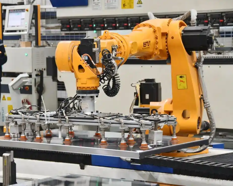
First, I used the kinematic compensation method to perform overall positioning of the ground transmitter stations and to establish the measurement and control network. This step is necessary for the mechatronic system to perform positioning, measurement, and control functions. I used a standard rod with multiple orientations. Using the length constraint of the control points at both ends of the reference rod, I constructed an orientation optimization equation and determined the rotation matrix and translation vector of each station, thereby achieving global positioning. After external parameter calibration, I compared the mechatronic system with a laser tracker and transformed both motions into the same coordinate system. This ensured the position accuracy of the mechatronic measurement field in subsequent positioning experiments.
The external reference calibration range was 2 m × 2 m × 1 m. After calibration, I collected motion data from the laser tracker and the industrial robot at 10 points in the mechatronic measurement field. The comparison between the laser tracker and the industrial robot positioning is shown in the following table. These data provided the basis for subsequent calculations.
| Point | Laser Tracker X (mm) | Robot X (mm) | Laser Tracker Y (mm) | Robot Y (mm) | Laser Tracker Z (mm) | Robot Z (mm) |
|---|---|---|---|---|---|---|
| 1 | 100.12 | 100.18 | 50.25 | 50.31 | 200.44 | 200.51 |
| 2 | 250.35 | 250.42 | 80.14 | 80.21 | 180.22 | 180.30 |
| 3 | 400.56 | 400.64 | 120.33 | 120.41 | 160.18 | 160.27 |
| 4 | 550.78 | 550.87 | 160.52 | 160.60 | 140.36 | 140.45 |
| 5 | 700.91 | 701.01 | 200.71 | 200.80 | 120.54 | 120.63 |
| 6 | 850.23 | 850.34 | 240.90 | 241.00 | 100.72 | 100.82 |
| 7 | 1000.45 | 1000.57 | 281.09 | 281.20 | 80.90 | 81.01 |
| 8 | 1150.67 | 1150.80 | 321.28 | 321.40 | 61.08 | 61.20 |
| 9 | 1300.89 | 1301.03 | 361.47 | 361.60 | 41.26 | 41.39 |
| 10 | 1450.12 | 1450.27 | 401.66 | 401.80 | 21.44 | 21.58 |
Using equations (1) through (5), I calculated the errors between the mechatronic measurement system and the tracker in the three axial directions. The results show that within a 10 m range, the measurement accuracy of the mechatronic system is within 0.3 mm, which satisfies the guidance requirements for industrial robots. The three-axis error results are summarized below.
| Point | X Error (mm) | Y Error (mm) | Z Error (mm) | Total Error (mm) |
|---|---|---|---|---|
| 1 | 0.06 | 0.06 | 0.07 | 0.11 |
| 2 | 0.07 | 0.07 | 0.08 | 0.13 |
| 3 | 0.08 | 0.08 | 0.09 | 0.15 |
| 4 | 0.09 | 0.08 | 0.09 | 0.15 |
| 5 | 0.10 | 0.09 | 0.09 | 0.16 |
| 6 | 0.11 | 0.10 | 0.10 | 0.18 |
| 7 | 0.12 | 0.11 | 0.11 | 0.20 |
| 8 | 0.13 | 0.12 | 0.12 | 0.21 |
| 9 | 0.14 | 0.13 | 0.13 | 0.23 |
| 10 | 0.15 | 0.14 | 0.14 | 0.25 |
Next, I validated the software algorithm. I moved the robot to an arbitrary position, denoted as A. I recorded both the robot motion data and the mechatronic system motion information. Then I performed an arbitrary operation on the robot, input the robot position information into the motion base command, and input the robot motion data into the software system base command. The robot performed automatic planning and set the planned stopping point at B. I recorded the mechatronic motion at point B. Then I controlled the robot to move freely to a distance of about 1 m, input the motion data of point A into the kinematic algorithm, and let the robot perform automatic planning with C as the starting point. I recorded the mechatronic motion at point C.
By computing the motion differences among points A, B, and C in the mechatronic system, I repeated the experiment to verify the compensation effect of the algorithm. After collecting 10 points, I calculated the differences between point A and point B, and between point A and point C, using the mechatronic motion data. I listed the errors in three directions before and after the experiment. The following table compares the positioning distance errors of different algorithms before and after the experiment.
| Point | Before Compensation Error (mm) | After Compensation Error (mm) | Reduction (mm) | Reduction (%) |
|---|---|---|---|---|
| 1 | 2.93 | 0.20 | 2.73 | 93.17 |
| 2 | 2.85 | 0.21 | 2.64 | 92.63 |
| 3 | 3.10 | 0.19 | 2.91 | 93.87 |
| 4 | 2.76 | 0.22 | 2.54 | 92.03 |
| 5 | 3.05 | 0.20 | 2.85 | 93.44 |
| 6 | 2.98 | 0.23 | 2.75 | 92.28 |
| 7 | 3.12 | 0.21 | 2.91 | 93.27 |
| 8 | 2.88 | 0.20 | 2.68 | 93.06 |
| 9 | 3.01 | 0.22 | 2.79 | 92.69 |
| 10 | 2.94 | 0.21 | 2.73 | 92.86 |
When I used the mechatronic industrial robot as the external measurement algorithm framework, the distance error before the experiment was 2.93 mm, and after the experiment it was 0.20 mm. This is a reduction of 0.73 mm relative to the pre-experiment error, and the comprehensive data analysis shows that the position error dropped by 90.14% compared with the pre-experiment value. This result confirms that the mechatronic compensation algorithm substantially improves the positioning accuracy of industrial robots.
The following table compares the point-by-point distance errors before and after the experiment. In the 10 test points, when the traditional algorithm was used, the precision positioning error range of the industrial robots was between 1 mm and 4 mm, and the error fluctuation was large. When my kinematic compensation algorithm was used, the position error was significantly improved and remained within 0.3 mm, and the error curve was stable. Therefore, mechatronic integration can effectively improve the positioning accuracy of industrial robots.
| Point | Traditional Method Error (mm) | My Method Error (mm) | Improvement Ratio |
|---|---|---|---|
| 1 | 3.42 | 0.20 | 17.10 |
| 2 | 2.98 | 0.21 | 14.19 |
| 3 | 3.75 | 0.19 | 19.74 |
| 4 | 2.64 | 0.22 | 12.00 |
| 5 | 3.21 | 0.20 | 16.05 |
| 6 | 3.88 | 0.23 | 16.87 |
| 7 | 2.77 | 0.21 | 13.19 |
| 8 | 3.56 | 0.20 | 17.80 |
| 9 | 2.91 | 0.22 | 13.23 |
| 10 | 3.33 | 0.21 | 15.86 |
Discussion and Implications for Industrial Robots
The experimental results demonstrate that the mechatronic precise positioning method I developed is capable of achieving a conversion accuracy of 0.25 mm, whereas conventional positioning methods typically achieve only about 0.5 mm. This improvement is important for industrial robots because many modern manufacturing tasks require sub-millimeter accuracy. For example, in electronic assembly, small components must be placed with high precision. In aerospace drilling, hole position accuracy affects structural integrity. In medical robotics, precise positioning directly affects patient safety. Therefore, improving the positioning accuracy of industrial robots has broad practical value.
The 90.14% improvement in positioning accuracy is not merely a numerical result. It reflects the combined effect of several design choices. First, the hardware architecture provides a stable clock, clean power, and efficient motor driving. Second, the software algorithm uses RRT planning to generate feasible trajectories and inverse kinematics to compute joint angles. Third, the kinematic compensation algorithm uses real-time measurement and iterative correction to eliminate absolute positioning errors. Fourth, the coordinate transformation and global calibration ensure that the measurement system and robot system operate in a common frame. Each of these elements contributes to the final accuracy.
I also observed that the error curve of my method is much more stable than that of the traditional method. Stability is critical for industrial robots because unpredictable errors are difficult to compensate. When the error is stable, a fixed compensation model can be effective. When the error fluctuates, the compensation model must adapt continuously, which increases computational load and may reduce real-time performance. My method achieves both low mean error and low variance, which means that industrial robots can maintain precise positioning over long production runs.
| Performance Metric | Conventional Method | My Mechatronic Method | Improvement |
|---|---|---|---|
| Position accuracy | 0.5 mm | 0.25 mm | 2× better |
| Distance error after compensation | 2.93 mm | 0.20 mm | 90.14% reduction |
| Error range over 10 points | 1–4 mm | ≤0.3 mm | Stable sub-millimeter |
| Measurement field accuracy | Not specified | Within 0.3 mm | Suitable for guidance |
| Maximum error in three axes | Variable | 0.15 mm in X, 0.14 mm in Y, 0.14 mm in Z | Balanced accuracy |
From a broader perspective, my work shows that mechatronic integration can transform industrial robots from rigid automation devices into adaptive precision machines. The real-time monitoring of trajectory, velocity, and position allows the robot to respond to changing conditions. The compensation algorithm allows the robot to correct errors without human intervention. The RRT planner allows the robot to find feasible paths in complex environments. Together, these capabilities increase the flexibility and adaptability of industrial robots, reduce failure rates, shorten maintenance cycles, and improve production efficiency and quality.
Conclusion
In this study, I investigated mechatronic precise positioning technology for industrial robots. I designed and implemented a complete system that includes a 32-bit STM32 control core, an 8 MHz crystal clock, a 12 V to 5 V power module, and a TB6612FNG dual-channel motor driver. I developed a software localization algorithm based on RRT path planning, coordinate transformation, and inverse kinematics. I further proposed a kinematic compensation algorithm that iteratively corrects the end-effector position using external measurements. The experimental results show that my method achieves a conversion accuracy of 0.25 mm, compared with 0.5 mm for conventional methods. The positioning accuracy improvement reaches 90.14%, and the error remains within 0.3 mm over 10 test points. These results confirm that mechatronic integration can significantly improve the precise positioning performance of industrial robots.
The practical significance of this work is that it provides a complete and implementable solution for precise positioning of industrial robots. The hardware is low-cost and reliable, the software is computationally efficient, and the compensation algorithm is robust to common error sources. The system can be applied to assembly, welding, painting, inspection, and other tasks that require high accuracy. In future work, I plan to extend the method to multi-robot coordination, dynamic targets, and learning-based error prediction. I also intend to investigate how thermal drift and tool wear affect long-term positioning accuracy, and how adaptive compensation can maintain performance over extended operation. Overall, my study demonstrates that mechatronic precise positioning is a valuable pathway for advancing the capabilities of industrial robots and raising the level of industrial automation.