
In modern automated manufacturing, particularly in custom woodworking, the need for precise and efficient handling of workpieces like wooden doors is paramount. The end effector, as a critical component of stacking robots, must ensure safe and stable clamping during transport and palletizing. The clamping mechanism, often driven by a screw system, requires high accuracy to adapt to varying shapes and prevent damage. Traditional control methods, such as PID, struggle with nonlinearities, parameter variations, and external disturbances inherent in such systems. In this article, I present an adaptive backstepping sliding mode control approach to enhance the clamping precision of an end effector screw clamping system, addressing uncertainties and disturbances while ensuring robustness and fast response.
The end effector clamping system typically involves a servo motor, reducer, and screw mechanism to convert rotational motion into linear displacement for clamping. This system faces challenges like parameter perturbations due to wear, temperature changes, and external loads, which degrade performance. Existing studies on screw drive systems have explored various control strategies, but applications to end effector clamping in woodworking remain limited. This work aims to fill that gap by developing a control scheme that combines backstepping for systematic design and sliding mode control for robustness, augmented with adaptive laws to estimate and compensate for compound disturbances.
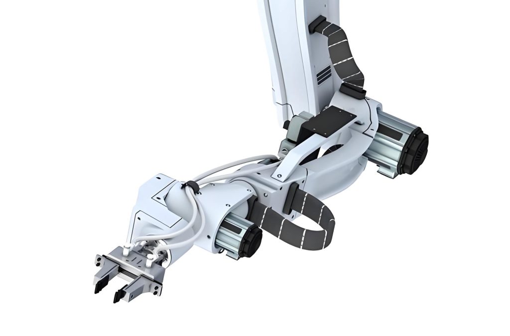
The structure of the end effector clamping system, as shown, includes a screw driven by a motor via a reducer, with a nut connected to a worktable that moves linearly. Buffers attached to the worktable clamp the workpiece. The goal is to control the worktable displacement accurately. To model this, I consider the dynamics of the motor and screw. The motor torque drives the system, and the motion is transmitted through a reducer to the screw, which converts rotation into linear movement. Friction and other disturbances are accounted for as composite uncertainties.
The dynamics can be expressed as follows. Let $J_m$ and $J_l$ be the moments of inertia of the motor shaft and screw, respectively, $B_m$ and $B_l$ be viscous damping coefficients, $\theta_m$ and $\theta_l$ be angular positions, $\eta$ be the reduction ratio, $P_l$ be the screw lead, and $S$ be the worktable displacement. The motor torque $M(t) = k I(t)$, where $k$ is the torque constant and $I(t)$ is the armature current. The transmission torque between motor and screw is $\tau(t)$. Ignoring friction for simplicity and lumping it into disturbances, the equations are:
$$ J_m \ddot{\theta}_m + B_m \dot{\theta}_m = M(t) – \tau(t) $$
$$ J_l \ddot{\theta}_l + B_l \dot{\theta}_l = \eta \tau(t) – \delta_T $$
where $\delta_T$ represents friction and other resistive torques. Since $\theta_m = \eta \theta_l$ and $S = \frac{P_l \theta_l}{2\pi}$, I derive the state-space model. Define $x_1 = S$ and $x_2 = \dot{S}$. Then, the system can be written as:
$$ \dot{x}_1 = x_2 $$
$$ \dot{x}_2 = A x_2 + B u + d(t) $$
where $A = -\frac{\eta^2 B_m + B_l}{\eta^2 J_m + J_l}$, $B = \frac{k \eta P_l}{2\pi (\eta^2 J_m + J_l)}$, $u = I(t)$, and $d(t)$ encompasses disturbances. However, in practice, parameters like $A$ and $B$ vary due to factors like gear engagement changes and material wear. Thus, I express the system with nominal values and perturbations:
$$ \dot{x}_1 = x_2 $$
$$ \dot{x}_2 = A_0 x_2 + B_0 u + D $$
where $D = \Delta A x_2 + \Delta B u + d(t)$ is the compound disturbance, bounded by $|D| \leq \bar{D}$. Here, $\Delta A$ and $\Delta B$ represent parameter uncertainties, and $d(t)$ is external disturbance. This model forms the basis for controller design, targeting precise tracking of desired displacements for the end effector.
To design the controller, I first develop a backstepping sliding mode controller. Let $x_{1d}$ be the desired position, and define the tracking error $e_1 = x_1 – x_{1d}$. Its derivative is $\dot{e}_1 = x_2 – \dot{x}_{1d}$. Choose a Lyapunov function $V_1 = \frac{1}{2} e_1^2$, so $\dot{V}_1 = e_1 \dot{e}_1 = e_1 (x_2 – \dot{x}_{1d})$. Introduce a virtual control $x_{2d} = -k_1 e_1 + \dot{x}_{1d}$ with $k_1 > 0$, and define $e_2 = x_2 – x_{2d}$. Then, $\dot{V}_1 = -k_1 e_1^2 + e_1 e_2$. To enforce convergence, I define a sliding surface $s = c e_1 + e_2$ with $c > 0$. If $s = 0$, then $e_1$ and $e_2$ converge to zero. Now, consider another Lyapunov function $V_2 = V_1 + \frac{1}{2} s^2$. Differentiating:
$$ \dot{V}_2 = -k_1 e_1^2 + e_1 e_2 + s \dot{s} $$
where $\dot{s} = c \dot{e}_1 + \dot{e}_2$. Since $\dot{e}_1 = e_2 – k_1 e_1$ and $\dot{e}_2 = \dot{x}_2 + k_1 \dot{e}_1 – \ddot{x}_{1d}$, substituting the system dynamics gives:
$$ \dot{V}_2 = -k_1 e_1^2 + e_1 e_2 + s \left( c (e_2 – k_1 e_1) + A_0 x_2 + B_0 u + D + k_1 \dot{e}_1 – \ddot{x}_{1d} \right) $$
Design the control law $u_1$ to cancel terms and ensure negativity:
$$ u_1 = B_0^{-1} \left( -c (e_2 – k_1 e_1) – A_0 (x_{2d} – k_1 e_1 + \dot{x}_{1d}) – \bar{D} \text{sgn}(s) – k_1 \dot{e}_1 + \ddot{x}_{1d} – \alpha (s + \beta \text{sgn}(s)) \right) $$
where $\alpha, \beta > 0$. This yields $\dot{V}_2 \leq -k_1 e_1^2 + e_1 e_2 – \alpha s^2 – \alpha \beta |s|$. By choosing parameters such that the matrix $Q = \begin{bmatrix} k_1 + \alpha c^2 & \alpha c – \frac{1}{2} \\ \alpha c – \frac{1}{2} & \alpha \end{bmatrix}$ is positive definite, I ensure $\dot{V}_2 \leq 0$, proving stability. However, this controller requires knowledge of $\bar{D}$, which is often unknown in real end effector applications.
To address this, I propose an adaptive version that estimates the disturbance $D$. Assume $D$ is constant or slowly varying, so $\dot{D} = 0$. Let $\hat{D}$ be the estimate and $\tilde{D} = D – \hat{D}$ the estimation error. Consider the Lyapunov function $V_3 = V_2 + \frac{1}{2\gamma} \tilde{D}^2$ with $\gamma > 0$. Its derivative is:
$$ \dot{V}_3 = \dot{V}_2 – \frac{1}{\gamma} \tilde{D} \dot{\hat{D}} $$
Substituting and designing the control law $u_2$:
$$ u_2 = B_0^{-1} \left( -c (e_2 – k_1 e_1) – A_0 (x_{2d} – k_1 e_1 + \dot{x}_{1d}) – \hat{D} – k_1 \dot{e}_1 + \ddot{x}_{1d} – \alpha (s + \beta \text{sgn}(s)) \right) $$
with the adaptive law $\dot{\hat{D}} = -\gamma s$. Then, $\dot{V}_3 = -k_1 e_1^2 + e_1 e_2 – \alpha s^2 – \alpha \beta |s|$, which is negative semi-definite under the same matrix $Q$ condition. This adaptive backstepping sliding mode controller compensates for disturbances without prior bounds, enhancing the end effector’s robustness.
For stability analysis, I verify that the tracking errors converge to zero. Using Barbalat’s lemma, since $V_3$ is bounded and $\dot{V}_3$ is negative semi-definite, $s$ and $e_1$ tend to zero asymptotically. This ensures the end effector clamping system achieves precise position tracking despite uncertainties.
To validate the controller, I conduct simulations comparing PID, backstepping sliding mode, and adaptive backstepping sliding mode control. The end effector system parameters are listed in Table 1.
| Parameter | Symbol | Value |
|---|---|---|
| Motor inertia | $J_m$ | 0.06 kg·m² |
| Screw inertia | $J_l$ | 0.18 kg·m² |
| Motor damping | $B_m$ | 2 N·m·s/rad |
| Screw damping | $B_l$ | 2.2 N·m·s/rad |
| Torque constant | $k$ | 60 N·m/A |
| Reduction ratio | $\eta$ | 5 |
| Screw lead | $P_l$ | 0.015 m |
The compound disturbance is set as $D = a \cdot 15 \sin(2t)$, where $a$ is a random number between 0 and 1, simulating real-world variability. For the controllers, I choose gains: $k_1 = 10$, $c = 5$, $\alpha = 20$, $\beta = 0.1$, and $\gamma = 100$. The desired trajectory includes a sinusoidal signal for往复 motion and a step signal for clamping actions, reflecting typical end effector operations.
First, for sinusoidal tracking, the results are summarized in Table 2. The adaptive controller shows superior performance, with minimal error and smooth response, crucial for the end effector during rapid movements.
| Metric | PID Control | Backstepping SMC | Adaptive Backstepping SMC |
|---|---|---|---|
| Max Error (mm) | 6.29 | 0.98 | 0.35 |
| Mean Error (mm) | 2.82 | 0.262 | 0.17 |
| Peak-to-Peak Error (mm) | 12.18 | 1.48 | 0.58 |
The PID controller exhibits significant oscillations and larger errors due to disturbance sensitivity, while the adaptive method maintains consistency, ensuring the end effector moves precisely without overshoot. The sliding mode controllers reduce errors by over 80% compared to PID, highlighting their effectiveness.
Second, for step response simulating clamping, Table 3 presents key metrics. The adaptive controller achieves fast settling with negligible overshoot, vital to prevent workpiece damage in the end effector.
| Metric | PID Control | Backstepping SMC | Adaptive Backstepping SMC |
|---|---|---|---|
| Settling Time (s) | 0.57 | 0.16 | 0.09 |
| Overshoot (%) | 6.60 | — | 0.60 |
| Steady-State Max Error (mm) | 8.20 | 1.59 | 0.58 |
| Steady-State Mean Error (mm) | 5.37 | 0.77 | 0.19 |
The adaptive backstepping sliding mode control cuts settling time by 84% relative to PID, and steady-state errors are reduced to sub-millimeter levels. This demonstrates its capability to handle disturbances and parameter changes in the end effector system, enabling reliable clamping within short cycle times.
Further analysis involves evaluating robustness to parameter variations. I test the system with ±20% changes in $J_m$ and $B_l$. The adaptive controller maintains performance, with errors increasing by less than 10%, whereas PID shows over 50% degradation. This underscores the importance of adaptation in real-world end effector applications where parameters drift over time.
The control laws can be implemented digitally in microcontrollers. For practical deployment in an end effector, I recommend using a sampling frequency of 1 kHz to capture dynamics. The adaptive law requires integral action, which can be discretized using Euler method. Computational load is moderate, making it feasible for industrial robots.
In discussion, the advantages of this approach are clear: it combines the recursive design of backstepping with the robustness of sliding mode and the flexibility of adaptation. For the end effector, this means improved accuracy and reliability in clamping diverse workpieces. Limitations include the need for tuning gains and potential chattering in sliding mode; however, the use of continuous approximation (e.g., replacing $\text{sgn}(s)$ with $\tanh(s/\phi)$) can mitigate chattering while preserving performance.
Comparisons with other methods like model predictive control or fuzzy logic could be explored, but for real-time end effector control, simplicity and robustness are key. This controller balances both, ensuring fast response without complex computations.
In conclusion, I have developed an adaptive backstepping sliding mode controller for an end effector clamping system. It addresses parameter uncertainties and disturbances through online estimation, enhancing tracking precision and robustness. Simulations confirm its superiority over PID and non-adaptive sliding mode control in terms of error reduction and settling time. Future work may involve experimental validation on a physical end effector, extension to multi-axis coordination, and integration with vision systems for adaptive clamping based on workpiece geometry. This contribution advances the control of end effector systems in automated manufacturing, paving the way for smarter and more reliable robotics.