
In the pursuit of higher precision and reliability for complex mechanical devices such as spacecraft and robots, which often incorporate harmonic drive gear systems as key reduction and torque amplification components, the accurate dynamic modeling of these systems has become a focal point of contemporary research. As a researcher deeply involved in this field, I have observed that harmonic drive gear systems operate on the principle of elastic deformation, primarily through the flexspline, leading to complex nonlinear dynamic behaviors. These behaviors significantly degrade transmission performance, manifesting as kinematic errors, friction-induced losses, nonlinear stiffness, and hysteresis effects. This article aims to comprehensively review the dynamic behaviors and associated modeling approaches for harmonic drive gear systems, emphasizing the use of tables and mathematical formulations to encapsulate key concepts. The term “harmonic drive gear” will be recurrently highlighted to underscore its centrality in this discussion.
Harmonic drive gear systems are renowned for their compact design, high reduction ratios, and zero-backlash operation, making them indispensable in precision applications. However, their inherent flexibility introduces challenges in dynamic modeling. The core dynamic behaviors—kinematic error, friction, nonlinear stiffness, and hysteresis—are intertwined, often coupling to produce detrimental effects on positioning accuracy, energy efficiency, and system stability. Over the years, numerous models have been developed to capture these phenomena, ranging from simple trigonometric representations to sophisticated hysteresis-based formulations. In this exposition, I will delve into the sources, characteristics, and impacts of these behaviors, followed by a detailed analysis of prevalent dynamic models. The integration of formulas and comparative tables will facilitate a clearer understanding of each model’s structure, advantages, and limitations.
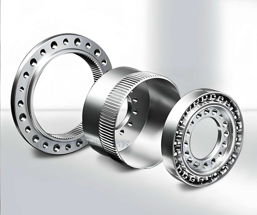
The illustration above provides a visual reference for a typical harmonic drive gear assembly, highlighting the interaction between the wave generator, flexspline, and circular spline. This interaction is fundamental to the dynamic behaviors discussed herein.
Dynamic Behaviors in Harmonic Drive Gear Systems
The dynamic performance of harmonic drive gear systems is governed by several nonlinear phenomena. Understanding these behaviors is crucial for developing accurate models.
Kinematic Error
Kinematic error in harmonic drive gear systems is defined as the deviation between the ideal and actual output angular displacements. For a system with input angular displacement \(\theta_i\), output angular displacement \(\theta_o\), and reduction ratio \(N\), the kinematic error \(\theta_e\) is expressed as:
$$ \theta_e = -\frac{\theta_i}{N} – \theta_o. $$
This error comprises two primary components: a periodic component stemming from manufacturing and assembly imperfections, and a high-frequency stochastic component induced by system compliance. The periodic error typically oscillates at twice the rotational frequency of the wave generator, as illustrated in the following table summarizing its sources and properties:
| Source | Characteristics | Impact on Transmission |
|---|---|---|
| Misalignment of components (e.g., circular spline axis offset) | Periodic, amplitude dependent on assembly depth | Static position error, variable instantaneous transmission ratio |
| Gear tooth profile inaccuracies | Periodic, frequency related to tooth engagement | Increased vibration and noise |
| System compliance under low torque | Stochastic, high-frequency | Speed fluctuations, reduced dynamic accuracy |
The stochastic component arises due to the nonlinear stiffness of the harmonic drive gear, which allows relative motion between the wave generator and flexspline at low torque levels. Factors influencing kinematic error include wave generator insertion depth, input speed, and load torque. Generally, increasing insertion depth reduces error amplitude, higher speeds amplify stochastic effects, and larger loads diminish error magnitude. The kinematic error directly affects both static and dynamic transmission performance, leading to positioning inaccuracies and resonant vibrations that exacerbate output speed variations.
Friction
Friction in harmonic drive gear systems originates from multiple contact regions: the interface between the wave generator’s flexible bearing and the flexspline inner wall, the meshing zone between the circular spline and flexspline teeth, and the output shaft bearings. For modeling purposes, the meshing zone friction is often predominant, as it contributes significantly to energy loss and hysteresis. Friction torque in harmonic drive gear systems exhibits a nonlinear relationship with input angular velocity and a periodic dependence on input angular displacement. Experimental studies show that friction torque initially increases with speed, then decreases, following a Stribeck-like curve. The effects of friction are profound: it accounts for substantial power dissipation and, when coupled with system flexibility, induces hysteresis in the stiffness curve, further degrading positional precision. The following equation typifies the nonlinear velocity dependence:
$$ T_{fr} = f(\dot{\theta}_i, \theta_i), $$
where \(T_{fr}\) is the friction torque, \(\dot{\theta}_i\) is the input angular velocity, and \(\theta_i\) is the input angular displacement. The periodic nature stems from the cyclic engagement of gear teeth over one revolution.
Nonlinear Stiffness and Hysteresis
The compliance of harmonic drive gear systems, primarily due to the flexspline and wave generator flexibility, results in nonlinear stiffness behavior. This means the torsional stiffness \(K\) is not constant but varies with transmitted torque \(T\):
$$ K = \frac{dT}{d\theta}, $$
where \(\theta\) is the angular deformation. Typically, stiffness hardens with increasing torque. Moreover, when combined with friction, the system exhibits hysteresis—a lag between torque and deformation that forms loop-like curves during loading and unloading cycles. This hysteresis is a memory-dependent phenomenon, where the current state depends on the history of deformation. The hysteresis loop characteristics are influenced by pre-sliding friction behavior at the tooth interfaces and driving conditions. The impact of nonlinear stiffness and hysteresis includes altered energy storage mechanisms, coupling with kinematic error to cause high-frequency stochastic errors, and reduced output position accuracy due to residual deformations. The table below summarizes key aspects:
| Behavior | Primary Source | Effect on Harmonic Drive Gear Performance |
|---|---|---|
| Nonlinear Stiffness | Elastic deformation of flexspline and wave generator | Variable natural frequency, torque-dependent compliance |
| Hysteresis | Coupling of friction and compliance | Energy dissipation, reduced positional accuracy, memory effects |
Dynamic Models for Harmonic Drive Gear Systems
To capture the aforementioned behaviors, various dynamic models have been proposed. These models range from simplistic to highly detailed, each with specific applicability. I will categorize them into kinematic error models, friction models, nonlinear stiffness models, and hysteresis stiffness models.
Kinematic Error Models
Kinematic error models aim to predict the discrepancy between ideal and actual motion. Two prominent types are trigonometric models and Lagrangian-based models.
Trigonometric Model: This model approximates the periodic component of kinematic error as a sum of sinusoidal functions or a Fourier series. It is simple but ignores stochastic components. The general form is:
$$ \theta_e = \sum_{t=1}^{n} A_t \sin(B_t \theta_i + \phi_t), $$
where \(A_t\), \(B_t\), and \(\phi_t\) are amplitude, angular frequency, and phase of the \(t\)-th harmonic, identified via spectral analysis. Its simplicity facilitates easy parameter identification, but it is unsuitable for high-precision applications where stochastic errors matter.
Lagrangian Model: This model incorporates system compliance and friction to account for both periodic and stochastic errors. Using generalized coordinates \(\theta_i\) and \(\theta_o\), the kinetic energy \(E\), potential energy \(V\), and Rayleigh dissipation function \(\Psi\) are formulated. For a harmonic drive gear system with lumped inertias \(J_i\) and \(J_o\), and stiffness modeled via a nonlinear function \(T(\theta)\), we have:
$$ E = \frac{1}{2} J_i \dot{\theta}_i^2 + \frac{1}{2} J_o \dot{\theta}_o^2, $$
$$ V = \int_0^{\theta_{e\_stiff}} T(\theta) d\theta, \quad \text{with } \theta_{e\_stiff} = \theta_o + \frac{\theta_i}{N} + \theta_{e\_cyc}, $$
where \(\theta_{e\_cyc}\) is the periodic error and \(\theta_{e\_stiff}\) is the stiffness-dependent error. The dissipation function includes viscous friction terms. Applying Lagrange’s equation yields the system dynamics. This model is more accurate but requires solving partial differential equations, making it computationally intensive.
| Model Type | Formulation | Advantages | Limitations |
|---|---|---|---|
| Trigonometric | $$ \theta_e = \sum A_t \sin(B_t \theta_i + \phi_t) $$ | Simple, easy parameter identification | Ignores stochastic errors, limited accuracy |
| Lagrangian | Based on energy functions and generalized coordinates | Captures compliance-induced stochastic errors | Computationally complex, requires friction modeling |
Friction Models
Friction models for harmonic drive gear systems can be static or dynamic. Static models, like Coulomb and viscous friction, are simplistic. Dynamic models, such as the LuGre model, better capture presliding and Stribeck effects.
LuGre Friction Model Applied to Harmonic Drive Gear: This model represents friction torque \(T_{fr}\) as a sum of a nonlinear velocity-dependent term \(T_{fr\_non}\) and a periodic displacement-dependent term \(T_{fr\_cyc}\):
$$ T_{fr} = T_{fr\_non} + T_{fr\_cyc}. $$
The nonlinear term uses a state variable \(z\) for average bristle deflection:
$$ \frac{dz}{dt} = \dot{\theta}_i – \frac{|\dot{\theta}_i|}{g(\dot{\theta}_i)} z, \quad g(\dot{\theta}_i) = \frac{1}{\sigma_0} \left[ F_c + (F_s – F_c) e^{-(\dot{\theta}_i / \omega)^2} \right], $$
where \(\sigma_0\) is bristle stiffness, \(F_c\) is Coulomb friction, \(F_s\) is static friction, and \(\omega\) is Stribeck velocity. Then,
$$ T_{fr\_non} = \sigma_0 z + \sigma_1 \dot{z} + \sigma_2 \dot{\theta}_i, $$
with \(\sigma_1\) and \(\sigma_2\) as damping coefficients. The periodic term is:
$$ T_{fr\_cyc} = (A + B \dot{\theta}_i) \sum_{t=1}^{n} \left[ a_t \cos(t \theta_i) + b_t \sin(t \theta_i) \right]. $$
This model effectively describes dynamic friction but may inaccurately represent hysteresis due to its linear bristle assumption.
Nonlinear Stiffness Models
These models describe the relationship between transmitted torque \(T\) and angular deformation \(\theta\), often measured at the flexspline. For a harmonic drive gear, \(\theta\) is defined as:
$$ \theta = \theta_{fo} – \theta_{fi} \approx \theta_{fo} + \frac{\theta_i}{N}, $$
assuming negligible wave generator deformation.
Piecewise Linear Model: This model approximates the stiffness curve with two or three linear segments, useful for bidirectional motion:
$$ T = \begin{cases}
k_1 \theta, & |\theta| \leq \theta_{thr} \\
k_1 \theta + k_2 \left[ \theta – \theta_{thr} \text{sgn}(\theta) \right], & |\theta| > \theta_{thr}
\end{cases}, $$
where \(k_1, k_2\) are slopes and \(\theta_{thr}\) is a threshold. It is simple but has discontinuous derivatives at thresholds.
Cubic Polynomial Model: A smooth representation suitable for unidirectional operation:
$$ T = a_1 \theta + a_3 \theta^3, $$
with coefficients \(a_1, a_3\). This avoids discontinuities but cannot describe bidirectional hysteresis.
| Model | Mathematical Form | Applicability |
|---|---|---|
| Piecewise Linear | $$ T = \begin{cases} k_1 \theta & \text{for } |\theta| \leq \theta_{thr} \\ k_1 \theta + k_2 [\theta – \theta_{thr} \text{sgn}(\theta)] & \text{otherwise} \end{cases} $$ | Bidirectional motion, simple control design |
| Cubic Polynomial | $$ T = a_1 \theta + a_3 \theta^3 $$ | Unidirectional continuous operation, smooth stiffness |
Hysteresis Stiffness Models
Hysteresis models integrate friction and compliance to capture memory-dependent loops. Key approaches include memory models, Maxwell-based models, and multi-body models.
Memory Model: This model, based on system memory fading over time, expresses torque as a sum of nonlinear stiffness term \(T_{stiff}\) and a friction term \(T_{fri}\) that is a functional of deformation history:
$$ T = T_{stiff} + \int_0^t \Phi(t, \tau) \theta(\tau) d\tau, $$
with a memory kernel \(\Phi(u) = \sum A_t e^{-\alpha_t u}\). Assuming a single exponential, it reduces to:
$$ \frac{dT_{fri}}{dt} + \alpha \left| \frac{d\theta}{dt} \right| T_{fri} – A \frac{d\theta}{dt} = 0. $$
This model has few parameters but assumes memory decay, which may not always hold.
Maxwell Hysteresis Model: This model uses a parallel arrangement of massless block-spring units to simulate hysteretic friction. Each block \(i\) has stiffness \(\beta_i\) and Coulomb friction \(e_i\). The total torque is:
$$ T(t) = \sum_{i=1}^n T_i(\theta(t)), $$
where for each block,
$$ T_i = \begin{cases}
\beta_i (-\theta – \theta_i), & \text{if } |\beta_i (-\theta – \theta_i)| < e_i \text{ and } \dot{\theta}_i = 0 \\
e_i \text{sgn}(\dot{\theta}), & \text{otherwise, with } \theta_i = -\theta – (e_i / \beta_i) \text{sgn}(-\dot{\theta})
\end{cases}. $$
This captures presliding and memory without decay assumptions, but parameter identification is complex due to piecewise functions.
Multi-Body Compliance Model: This model accounts for flexibility in both the flexspline and wave generator. Defining angular deformations \(\theta_f\) for flexspline and \(\theta_w\) for wave generator, with stiffness functions:
$$ K_f = \frac{dT_f}{d\theta_f} = K_{f0} \left[ 1 + (C_f T_f)^2 \right], \quad K_w = \frac{dT_w}{d\theta_w} = K_{w0} e^{C_w T_w}, $$
the total deformation \(\theta\) becomes:
$$ \theta = \frac{\arctan(C_f T_f)}{C_f K_{f0}} – \frac{\text{sgn}(T_w)}{N C_w K_{w0}} \left( 1 – e^{-C_w |T_w|} \right), $$
with \(T_w = -\frac{1}{N}(T_f – T_{fr})\). This model incorporates wave generator effects but oversimplifies friction and assumes no relative motion between components.
| Hysteresis Model | Key Equations | Strengths | Weaknesses |
|---|---|---|---|
| Memory Model | $$ \frac{dT_{fri}}{dt} + \alpha \left| \frac{d\theta}{dt} \right| T_{fri} – A \frac{d\theta}{dt} = 0 $$ | Few parameters, captures fading memory | Assumes memory decay, may not fit all conditions |
| Maxwell Model | $$ T(t) = \sum T_i(\theta(t)) $$ with block-spring dynamics | Accurately models presliding hysteresis, no memory decay assumption | Complex parameter identification, piecewise functions |
| Multi-Body Model | $$ \theta = \frac{\arctan(C_f T_f)}{C_f K_{f0}} – \frac{\text{sgn}(T_w)}{N C_w K_{w0}} (1 – e^{-C_w |T_w|}) $$ | Includes wave generator compliance, simple form | Simplified friction, unrealistic assumptions about relative motion |
Summary and Future Perspectives
In reviewing the dynamic modeling of harmonic drive gear systems, it is evident that significant progress has been made in characterizing kinematic error, friction, nonlinear stiffness, and hysteresis. Models such as trigonometric and Lagrangian approaches for kinematic error, LuGre for friction, piecewise linear and cubic polynomial for stiffness, and memory, Maxwell, and multi-body models for hysteresis each offer unique advantages. However, challenges remain. The hysteresis stiffness model and compliance-dependent kinematic error model are particularly critical yet difficult to perfect due to the complex coupling between friction and flexibility.
Several areas warrant further investigation to enhance the accuracy and applicability of harmonic drive gear models. First, the generation mechanism of high-frequency stochastic kinematic error components needs deeper exploration. While Lagrangian models attribute it to system compliance, a more detailed analysis of flexspline deformation dynamics could yield better predictive models. Second, the coupling mechanism between flexibility and friction in harmonic drive gear systems requires clarification. Current hysteresis models often oversimplify friction behaviors, such as Stribeck effects, presliding displacement, and stick-slip phenomena at gear meshing interfaces. Future research should focus on experimentally characterizing these friction mechanisms and integrating them into comprehensive models. Additionally, the influence of wave generator flexibility and its interaction with other components merits more attention, as assumptions of no relative motion may not hold in practice.
Moreover, most existing models are phenomenological, derived from observed behaviors rather than first principles. Developing physics-based models that account for the detailed mechanics of harmonic drive gear components could improve generalizability across different designs and operating conditions. Another promising direction is the incorporation of advanced control strategies directly into dynamic models, enabling real-time compensation for nonlinearities and hysteresis in high-precision applications like space robotics and industrial automation.
In conclusion, the dynamic modeling of harmonic drive gear systems is a vibrant field essential for advancing precision engineering. By addressing the current limitations through mechanistic studies and innovative modeling approaches, we can achieve higher fidelity simulations, better control algorithms, and ultimately, more reliable and accurate harmonic drive gear-based devices. The continued emphasis on keyword aspects such as harmonic drive gear performance, harmonic drive gear hysteresis, and harmonic drive gear friction will drive future breakthroughs in this domain.
To encapsulate, the journey toward perfecting harmonic drive gear models involves balancing complexity with practicality, always aiming to capture the intricate dance of forces and motions that define these remarkable systems. As research progresses, the integration of data-driven techniques with physical models may offer new pathways, but the foundational understanding of dynamic behaviors will remain paramount.