
The advancement of collaborative robotics has spurred significant research into robotic systems for applications involving direct interaction with human skin, such as medical rehabilitation, massage, and aesthetic care. A paramount requirement in these applications is safety, which often necessitates the design of the robotic end effector to possess compliance or flexibility. This compliance allows the end effector to adapt to the contours and reactions of the skin, mitigating the risk of excessive force or injury. However, this very flexibility introduces a critical challenge: the precise determination of the contact point—or endpoint—of the end effector on the skin surface during operation. As the compliant element deforms under contact forces, the spatial location of its tip changes relative to the rigid base of the robot arm. Accurate real-time detection of this endpoint is fundamental for ensuring the precision of trajectory tracking, the consistency of the applied procedure, and overall operational safety. Without reliable endpoint detection, controlling the robot’s motion based solely on the arm’s kinematic model becomes inaccurate, potentially leading to ineffective or unsafe interactions.
Traditional computer vision methods for target point detection often struggle with the variability and unstructured nature of this task. Techniques relying on color markers are highly sensitive to lighting conditions and occlusion. Methods like Hough transforms are limited to detecting specific geometric shapes (lines, circles), which the end effector tip does not conform to during deformation. Edge detection and other feature-based approaches require extensive manual engineering to extract robust geometric features that can generalize across various deformation states and backgrounds, making them brittle in practical settings.
In recent years, deep learning-based approaches, particularly deep convolutional neural networks (CNNs), have revolutionized fields like human pose estimation and facial landmark detection. These methods learn hierarchical feature representations directly from data, offering superior accuracy and robustness compared to traditional techniques. Their ability to model complex non-linear relationships makes them ideally suited for detecting the endpoint of a deforming end effector from image data. However, a significant barrier to their adoption in industrial and specialized robotic applications is their insatiable demand for large, annotated datasets. State-of-the-art models in computer vision are typically trained on hundreds of thousands to millions of labeled images (e.g., MPII, COCO). Collecting and annotating such vast datasets for a specific task, such as detecting the tip of a particular flexible end effector, is often prohibitively expensive, time-consuming, and sometimes impractical.
This creates a core problem: how can we leverage the powerful representational capacity of deep learning for precise endpoint detection when only a small dataset is available for our specific target domain? The answer lies in transfer learning. The core idea is to transfer knowledge learned from a large, general-source dataset (e.g., ImageNet for object recognition) to a related but different target task with limited data. Instead of training a deep network from scratch with random initialization, we start with a model pre-trained on the source task. The underlying hypothesis is that the low-level and mid-level features learned by the early layers of the network—such as edges, textures, and simple shapes—are general and transferable across a wide range of visual tasks. We can then adapt or fine-tune the higher layers of this pre-trained model to specialize for our specific target task, such as endpoint regression for our flexible end effector. This approach dramatically reduces the amount of target-domain data required, accelerates convergence, and helps prevent overfitting, making deep learning viable for applications with small sample sizes.
This article presents a comprehensive methodology for detecting the endpoint of a compliant end effector using a deep transfer learning framework. We construct a regression network based on the powerful ResNet architecture. To effectively transfer knowledge, we employ a domain adaptation strategy that aligns the feature distributions between the source and target domains within the network’s hidden layers. This method allows us to train an accurate model using a remarkably small dataset of labeled images. We detail the experimental setup, including the design of the flexible end effector, the construction of the vision system, and the collection of the target dataset. Finally, we present quantitative results demonstrating the model’s precision in 2D pixel localization and its subsequent 3D spatial positioning accuracy for the end effector endpoint.
Deep Transfer Learning Model Architecture
Endpoint Regression Network Backbone
The foundation of our detection model is a deep residual network (ResNet). The introduction of ResNets addressed the degradation problem in very deep networks, where accuracy saturates and then degrades rapidly as depth increases. The key innovation is the residual block, which uses skip connections or identity mappings. Instead of hoping each stacked layer directly fits a desired underlying mapping, ResNets explicitly let these layers fit a residual mapping. Formally, if we denote the desired underlying mapping for a block as $H(x)$, the stacked nonlinear layers are designed to fit a different mapping: $F(x) := H(x) – x$. The original mapping thus becomes $H(x) = F(x) + x$. This structure, visualized in its basic form, is described by:
$$ \mathbf{y} = \mathcal{F}(\mathbf{x}, \{W_i\}) + \mathbf{x} $$
where $\mathbf{x}$ and $\mathbf{y}$ are the input and output vectors of the block, and the function $\mathcal{F}(\mathbf{x}, \{W_i\})$ represents the residual mapping to be learned (e.g., a sequence of convolution, batch normalization, and ReLU operations). The addition $+ \mathbf{x}$ is performed by a shortcut connection, which incurs no extra parameter or computational complexity. This design makes it significantly easier to train networks with hundreds of layers, as it mitigates the vanishing gradient problem.
We utilize the ResNet-50 variant as our backbone, which has proven to be an excellent trade-off between depth, computational cost, and performance. The architecture of ResNet-50 is structured into stages, as summarized in the table below:
| Layer Name | ResNet-50 Architecture |
|---|---|
| Conv1 | 7×7, 64, stride 2 |
| Max Pool | 3×3, stride 2 |
| Stage1 (Conv2_x) | $\begin{bmatrix} 1\times1, & 64 \\ 3\times3, & 64 \\ 1\times1, & 256 \end{bmatrix}$ × 3 |
| Stage2 (Conv3_x) | $\begin{bmatrix} 1\times1, & 128 \\ 3\times3, & 128 \\ 1\times1, & 512 \end{bmatrix}$ × 4 |
| Stage3 (Conv4_x) | $\begin{bmatrix} 1\times1, & 256 \\ 3\times3, & 256 \\ 1\times1, & 1024 \end{bmatrix}$ × 6 |
| Stage4 (Conv5_x) | $\begin{bmatrix} 1\times1, & 512 \\ 3\times3, & 512 \\ 1\times1, & 2048 \end{bmatrix}$ × 3 |
| Final Layers | Average Pool, 1000-d FC, Softmax (for classification) |
For our endpoint regression task, we repurpose this architecture. We remove the final classification-specific layers (the 1000-dimensional fully-connected layer and softmax). The ResNet-50 backbone up to the final average pooling layer serves as a powerful, generic feature extractor. We then append a new, task-specific regression head. This head consists of a fully-connected layer that maps the 2048-dimensional feature vector from the pool layer to a 2-dimensional output vector, representing the predicted $(u, v)$ pixel coordinates of the end effector endpoint. To obtain these coordinates directly, we apply an identity activation (linear activation). The network is trained to minimize the error between this prediction and the ground-truth labeled coordinates.
Domain Adaptive Transfer via Feature Alignment
While initializing our network with weights pre-trained on ImageNet provides a strong starting point, a simple fine-tuning approach on a very small target dataset may still be susceptible to overfitting or poor generalization. This is because the feature distributions of the source domain (general objects in ImageNet) and our target domain (images of a flexible end effector in contact with skin) can be substantially different. To bridge this “domain gap” more effectively, we incorporate an explicit domain adaptation strategy during transfer.
Our approach is inspired by feature-based domain adaptation methods. The core idea is to guide the learning process in the target network by encouraging its intermediate feature representations to align with those of the frozen source network (pre-trained on ImageNet). This is achieved by introducing an auxiliary adaptation loss at specific layers of the network.
Let $ \Phi $ represent the parameters of the pre-trained source model (ResNet-50 on ImageNet), which remain frozen. Let $ \Theta $ be the parameters of our target model (the endpoint regression network) that we are training. During the forward pass for a target domain image $a$, we process it through both networks in parallel. However, for the source network, we only forward propagate up to the selected adaptation layers to extract feature maps; we do not compute its final classification output.
We define a set of adaptation layers $m \in D$, typically chosen from the later convolutional stages (e.g., from Stage3 or Stage4) where features become more task-specific yet still transferable. For a given layer $m$, let $S^m_{\Phi}(a)$ be the feature map tensor from the frozen source network, and let $T^m_{\Theta}(a)$ be the corresponding feature map tensor from the trainable target network.
To align these features, we introduce a per-neuron, per-channel adaptation loss. For the $i$-th neuron (spatial location considered across channels) in layer $m$, and for each channel $j$, we compute a squared difference between the source feature and a linearly transformed target feature. A learnable channel-wise weight $ \omega^m_{i,j} $ determines the importance of aligning that specific feature channel. A linear transformation $r_{\Theta}$ (implemented as a 1×1 convolution without bias) is applied to the target features $T^m_{\Theta}(a)$ to project them into a space compatible for comparison with the source features, accounting for potential scale differences. The adaptation loss for neuron $i$ in layer $m$ is:
$$ \mathcal{L}_{m,i \in C}(\Theta | a, \omega^m_{i,j}) = \frac{1}{HW} \sum_{i,j \in d} \omega^m_{i,j} \left( r_{\Theta}(T^m_{\Theta}(a)_{i,j}) – S^m_{\Phi}(a)_{i,j} \right)^2 $$
where $C$ denotes the set of all neurons in the feature map, $H$ and $W$ are the spatial dimensions of the feature maps, and $d$ is the channel dimension. The total adaptation loss for layer $m$ is a weighted sum over all its neurons:
$$ \mathcal{L}_m(\Theta | a, \Phi) = \sum_{i \in C} \lambda^m_i \mathcal{L}_{m,i}(\Theta | a, \omega^m_{i,j}) $$
where $ \lambda^m_i $ is a positive scalar that controls the transfer strength for neuron $i$. The overall transfer loss for the model is the sum of these losses across all selected adaptation layers:
$$ \mathcal{L}_{transfer}(\Theta | a, \Phi) = \sum_{m \in D} \mathcal{L}_m(\Theta | a, \Phi) $$
Composite Loss Function for Training
The target model is trained to perform two simultaneous but complementary tasks: 1) accurately regressing the endpoint coordinates (the primary task), and 2) aligning its feature distributions with the source model to facilitate transfer (the auxiliary adaptation task). Therefore, the total loss function minimized during training is a composite of the primary regression loss and the feature alignment loss:
$$ \mathcal{L}_{total}(\Theta | a, b, \Phi) = \mathcal{L}_{tar}(\Theta | a, b) + \mathcal{L}_{transfer}(\Theta | a, \Phi) $$
Here, $b$ represents the ground-truth 2D coordinates for the input image $a$.
For the primary regression loss $ \mathcal{L}_{tar} $, we use the Smooth L1 Loss (also known as Huber loss for regression). This loss is less sensitive to outliers than the Mean Squared Error (MSE) and provides more stable gradients. It behaves like an L2 loss for small errors and like an L1 loss for larger errors, controlled by a threshold parameter $\delta$.
$$ \mathcal{L}_{tar}(\Theta | a, b) = \begin{cases}
\frac{1}{2}(b – f(a))^2, & \text{if } |b – f(a)| \leq \delta \\
\delta |b – f(a)| – \frac{1}{2}\delta^2, & \text{otherwise}
\end{cases} $$
where $f(a)$ is the 2D coordinate output of the target network parameterized by $\Theta$.
By minimizing $ \mathcal{L}_{total} $, the network learns to extract features from the target end effector images that are discriminative for endpoint localization (via $ \mathcal{L}_{tar} $) while simultaneously being grounded in the general visual concepts embedded in the pre-trained source model (via $ \mathcal{L}_{transfer} $). This combined objective is crucial for achieving robust performance with limited target data.
Experimental System and Data Preparation
Design and Characteristics of the Flexible End Effector
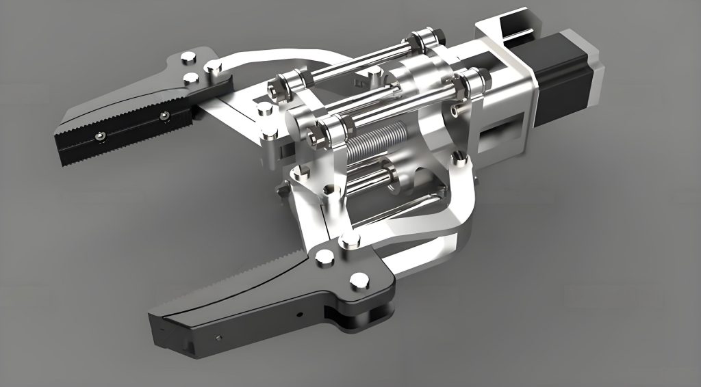
The focal point of this study is a custom-designed compliant end effector. Its primary function is to safely interact with human skin, requiring it to absorb and adapt to forces rather than transmitting them rigidly. The end effector is constructed in two distinct parts: a rigid base and an elastic, deformable tip component. The rigid base provides a stable mechanical interface for mounting onto the robot flange. The elastic tip is the interactive element; it is made from a material with a suitable durometer (e.g., silicone or soft thermoplastic elastomer) that allows for significant reversible deformation.
The key characteristic of this end effector is its ability to deform in multiple degrees of freedom upon contact. When an axial force is applied (pressing straight down), the tip compresses longitudinally. When a lateral or shear force is applied, the tip bends, causing an angular deflection. In a typical skin interaction scenario, such as moving across a curved surface like the face or scalp, the tip experiences a combination of these forces, leading to a complex, continuously changing deformation state. Crucially, the geometric tip point—the very endpoint we aim to detect—displaces from its nominal, non-contact position relative to the rigid base. This displacement is not easily modeled purely through robot kinematics or force sensors, making vision-based detection essential. The end effector‘s compliance ensures safety but creates the core perception challenge this work addresses.
Endpoint Detection and 3D Localization Platform
To validate our approach, we constructed a robotic experimental platform centered on a 6-axis collaborative robot arm (UR3e). The flexible end effector is mounted on the robot’s flange. The task scenario involves the robot maneuvering the end effector to make contact with a human head model, simulating a practical skin-interaction task.
Since controlling the robot requires knowledge of the endpoint’s position in 3D Cartesian space (not just 2D image coordinates), we employ a stereo vision system for 3D triangulation. The system consists of two calibrated cameras positioned to provide overlapping views of the workspace. The overall detection and localization pipeline follows these stages:
- Stereo Calibration: Using the Zhang’s method, we perform intrinsic and extrinsic calibration for both cameras. This process yields camera matrices, distortion coefficients, and, crucially, the relative rotation and translation between the two cameras. Rectification transforms are computed to align the image planes, simplifying the subsequent stereo correspondence problem to a search along horizontal epipolar lines.
- 2D Endpoint Detection: For each new stereo image pair, our trained deep transfer learning model processes the image from the primary (e.g., left) camera. The model outputs the predicted $(u_L, v_L)$ pixel coordinates of the end effector endpoint in the left image. A corresponding point in the right image $(u_R, v_R)$ is found using stereo matching techniques, constrained by the rectification. For a distinctive feature like a tip, simple block matching or more sophisticated algorithms can be used, aided by the small search range post-rectification.
- 3D Triangulation: Given the matched 2D points $(u_L, v_L)$ and $(u_R, v_R)$ and the calibrated camera projection matrices $P_L$ and $P_R$, the 3D world coordinate $(X, Y, Z)$ of the endpoint is reconstructed via linear triangulation methods, solving the equation $ \mathbf{x}_L \times (P_L \mathbf{X}) = 0 $ and $ \mathbf{x}_R \times (P_R \mathbf{X}) = 0 $ for the homogeneous 3D point $\mathbf{X}$.
This pipeline allows us to move from a raw stereo image pair to a precise 3D location of the flexible end effector‘s contact point, enabling closed-loop robotic control.
Dataset Collection and Curation
A critical component for training and evaluation is a dedicated dataset of the flexible end effector interacting with the target surface. We collected a dataset of 1000 unique images at a resolution of 480×480 pixels. The images capture the end effector in a wide variety of states:
- Varying Contact Locations: The robot was programmed to touch different areas of the head model (forehead, cheek, chin, scalp).
- Varying Contact Forces/Orientations: The robot approached the surface with different angles and slight variations in force, inducing the characteristic compressive and bending deformations of the tip.
- Varying Backgrounds and Lighting: While controlled, minor variations in ambient lighting and background clutter were present to add realism and encourage robustness.
Each image was meticulously annotated by manually labeling the precise pixel coordinates of the end effector endpoint (the tip). This ground-truth data is essential for training the regression model and evaluating its performance. To structure our experiments, particularly to investigate the effect of dataset size, we partitioned the full dataset into fixed subsets for training, validation, and testing. The validation set is used for hyperparameter tuning and monitoring for overfitting during training, while the test set is held out for a final, unbiased evaluation of the model’s generalization capability.
Experimental Results and Analysis
Model Training and the Impact of Dataset Size
To rigorously evaluate the efficacy of our transfer learning approach in a small-data regime, we designed an experiment with varying sizes of the training subset. The full dataset was partitioned with a 60%/20%/20% ratio for training, validation, and testing, respectively, resulting in 600 training, 200 validation, and 200 test images. We then created four distinct experimental groups by subsampling the training set:
| Experiment Group | Training Subset Size | Validation Subset Size | Test Subset Size |
|---|---|---|---|
| Group 1 | 300 | 100 | 100 |
| Group 2 | 400 | 120 | 120 |
| Group 3 | 500 | 150 | 150 |
| Group 4 (Full) | 600 | 200 | 200 |
The model was trained using stochastic gradient descent with momentum. A step-wise decaying learning rate schedule was employed, starting at 0.05 and reducing to 0.02, 0.002, and finally 0.001 at specified iteration milestones to ensure stable convergence. Weight decay (L2 regularization coefficient of 0.05) was used to prevent overfitting. Training was conducted for 50,000 iterations per group, as the loss curves were observed to plateau well before this point, indicating convergence. The smooth decrease and stabilization of the composite loss $ \mathcal{L}_{total} $ confirmed the stability of the training process with our transfer learning setup.
After training, we evaluated the model’s 2D detection accuracy on both the validation and test sets. The metric used is the average Euclidean distance (in pixels) between the predicted endpoint coordinates and the ground-truth coordinates across all images in the set. The results are compelling:
| Experiment Group | Validation Set Accuracy (pixels) | Test Set Accuracy (pixels) |
|---|---|---|
| Group 1 (300 images) | 13.4 | 15.6 |
| Group 2 (400 images) | 2.7 | 6.4 |
| Group 3 (500 images) | 2.4 | 5.8 |
| Group 4 (600 images) | 2.5 | 5.7 |
The results clearly demonstrate the power of transfer learning. Even with only 300 training images (Group 1), the model learns a meaningful mapping, though with higher error. There is a dramatic improvement in performance when increasing the training set to 400 images, with validation error dropping to 2.7 pixels. Most importantly, we observe that the performance begins to saturate at around 500 training images. The accuracy on the test set for Group 3 (5.8 pixels) is nearly identical to that of Group 4 (5.7 pixels), which used the full 600-image training set. This indicates that with our transfer learning framework, a dataset of approximately 500 annotated images is sufficient to train a model that achieves the maximal performance possible with this network architecture and data distribution. The small gap between validation and test error in Groups 3 and 4 also suggests good generalization without significant overfitting.
3D Endpoint Localization Accuracy
The ultimate measure of success for this system is its accuracy in determining the 3D spatial position of the end effector endpoint, as this coordinate is used for robot feedback control. Using the model trained on 500 images (Group 3), we conducted a comprehensive 3D localization experiment. The robot was commanded to position the end effector at five different, known locations within the workspace. At each location, we took 20 separate stereo image measurements, resulting in 100 independent 3D coordinate estimates in total.
For each measurement, we computed the absolute error along each world coordinate axis (X, Y, Z) as well as the overall 3D Euclidean error $ D = \sqrt{\Delta X^2 + \Delta Y^2 + \Delta Z^2} $. The following table summarizes the average absolute errors for each of the five test locations:
| Test Location | Avg. |ΔX| (mm) | Avg. |ΔY| (mm) | Avg. |ΔZ| (mm) | Avg. 3D Error |D| (mm) |
|---|---|---|---|---|
| Location 1 | 0.878 | 0.986 | 1.210 | 1.790 |
| Location 2 | 1.123 | 0.753 | 0.838 | 1.590 |
| Location 3 | 0.743 | 0.996 | 1.153 | 1.695 |
| Location 4 | 1.004 | 0.986 | 0.630 | 1.542 |
| Location 5 | 0.858 | 1.072 | 1.102 | 1.761 |
Aggregating across all 100 measurements, the mean 3D localization error $|\bar{D}|$ was 1.675 mm, with a standard deviation of 0.107 mm. This level of precision is highly significant for applications involving gentle skin contact, such as robotic massage or dermatological scanning. An error of under 2 mm is typically well within the tolerances required for such procedures, where the focus is on broad area coverage or consistent pressure application rather than micron-level accuracy. The consistency of the error across different spatial locations (as indicated by the low standard deviation) confirms the robustness of the vision system and the trained detection model. The system successfully translates the 2D pixel-level accuracy of the deep learning model into precise and reliable 3D coordinates for the deforming tip of the flexible end effector.
Conclusion
This work presents a practical and effective solution to a key perception problem in compliant robotics: detecting the endpoint of a flexible end effector under deformation. By formulating the problem as a direct coordinate regression task and employing a deep transfer learning strategy, we overcome the major barrier of requiring massive annotated datasets. The integration of a domain adaptation loss, which explicitly aligns feature distributions between a general-purpose pre-trained network and our specific target task, is crucial for achieving high performance with limited data. Our experiments empirically demonstrate that this approach enables the training of a robust detection model with a remarkably small dataset of around 500 images. The resulting system achieves a 3D endpoint localization accuracy of approximately 1.7 mm, which is sufficient for a wide range of human-interactive robotic applications where safety via compliance is paramount. The methodology is not limited to the specific end effector or task shown here; it provides a general framework for applying advanced deep learning techniques to specialized industrial and robotic vision problems where data scarcity is a fundamental constraint. Future work may involve extending the model to predict the endpoint in sequences of images (tracking), integrating the visual feedback directly into a force-visual servo controller, or adapting the approach to other deformable or articulated tools.