
I study visual servoing for industrial robots because the accuracy and robustness of the visual feedback loop directly determine the execution efficiency of industrial tasks. In my work, I treat the visual servo controller of industrial robots as a tightly coupled perception-and-action system. The perception side must recover a reliable six-dimensional pose from images that are often degraded by complex illumination, specular reflection, motion blur, and partial occlusion. The action side must convert that pose into joint-level motion commands that are stable, fast, and precise. When either side becomes unreliable, the closed loop of industrial robots loses stability, the end effector drifts away from the desired pose, and the task cycle time increases. Traditional image-based visual servoing, usually abbreviated as IBVS, relies on handcrafted feature points and a local interaction matrix. Although IBVS is mathematically elegant and computationally efficient, it tends to fail when the observed target is partially hidden or when the illumination changes abruptly. In such cases, feature extraction becomes noisy, the pose estimate becomes biased, and the controller of industrial robots must compensate for errors that are not physically meaningful.
I propose a deep learning visual servoing method for industrial robots that fuses a lightweight convolutional neural network with an IBVS architecture. The network extracts robust target features from grayscale images and regresses a six-dimensional pose vector. The pose vector is then converted into image-plane feature coordinates, and the classical IBVS control law drives the joints of industrial robots. I further design a pose error compensation formula and an adaptive speed control strategy. The compensation formula suppresses systematic calibration errors and random feature errors. The adaptive speed strategy changes the joint velocity according to the magnitude of the image-plane feature error, so industrial robots move quickly when the error is large and slowly when the error is small. I evaluate the method on a six-axis serial industrial robot under three representative scenarios: normal illumination without occlusion, weak illumination without occlusion, and normal illumination with partial occlusion. The experimental results show that my method keeps the position error below 0.07 mm and the orientation error below 0.05 degrees in all scenarios, while reducing the response time by more than 30 percent compared with traditional IBVS.
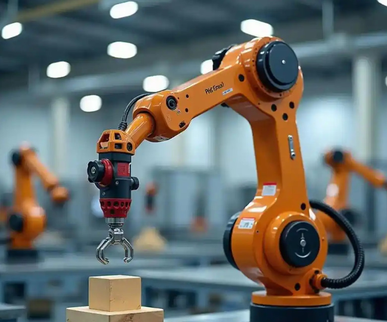
Introduction
Industrial robots are widely used in assembly, handling, polishing, inspection, and machine tending. In these applications, the robot must often locate a workpiece whose pose is not exactly known in advance. Vision is the most flexible sensing modality for this purpose, and visual servoing is the control framework that closes the loop between the camera and the motion of industrial robots. The core idea of visual servoing is to define an error in the image or in the pose space, and then to drive the robot so that the error converges to zero. IBVS defines the error directly in the image plane. This choice avoids the need for a perfect camera calibration and makes the controller robust to some calibration errors. However, IBVS still depends on reliable feature correspondence. If the feature points are extracted incorrectly, the interaction matrix maps the wrong error into the joint space, and the behavior of industrial robots becomes unpredictable.
Convolutional neural networks have changed the way I think about feature extraction for industrial robots. A deep network can learn hierarchical representations that are less sensitive to illumination changes and partial occlusion than handcrafted descriptors. The early layers capture edges, corners, and local texture. The deeper layers capture object-level structure. When I train such a network on images collected from the actual workspace of industrial robots, the network learns features that are aligned with the task rather than with a generic notion of visual saliency. This is especially important in industrial environments, where the background may contain metallic surfaces, conveyor belts, cables, and other objects that confuse classical detectors.
My motivation is practical. Industrial robots must operate continuously under lighting conditions that change with the time of day, the state of the factory windows, and the activation of nearby welding or inspection equipment. In many cells, the target is partially occluded by a gripper, a fixture, or another part. I have observed that under these conditions, a traditional IBVS pipeline can spend a large part of its cycle time correcting feature errors that originate from misdetection rather than from true motion. The result is slower convergence and, in the worst case, oscillation. A learning-based feature extractor can reduce this problem, but only if it is lightweight enough to run on an embedded controller or an industrial PC alongside the motion control loop. This constraint shapes my design: I do not use a large backbone that would require a data center GPU. Instead, I build a small network based on depthwise separable convolution and I remove the classification head entirely.
The contribution of my work can be summarized as follows. First, I design a lightweight convolutional neural network for industrial robots that takes a grayscale image and outputs a six-dimensional pose feature vector. Second, I integrate this network into an IBVS control architecture with a clear synchronization strategy between the vision thread and the motion thread. Third, I propose a pose error compensation formula that uses historical error feedback with exponential attenuation. Fourth, I propose an adaptive speed control strategy that maps the image-plane feature error norm to the joint velocity of industrial robots. Fifth, I validate the method on a real six-axis industrial robot and compare it with a traditional SIFT-based IBVS baseline under multiple illumination and occlusion conditions.
Problem Formulation and Notation
I formulate the visual servoing problem for industrial robots in the following way. Let the pose of the target relative to the camera be represented by a six-dimensional vector
$$
X = \begin{bmatrix} p_x & p_y & p_z & \theta_x & \theta_y & \theta_z \end{bmatrix}^{T}
$$
where the first three components describe position and the last three components describe orientation. The camera is mounted on the end effector of the industrial robot, forming an eye-in-hand configuration. The camera acquires an image at discrete time instants. At each instant, the network produces an estimate of the pose vector. Let the desired pose be
$$
X_d = \begin{bmatrix} p_{dx} & p_{dy} & p_{dz} & \theta_{dx} & \theta_{dy} & \theta_{dz} \end{bmatrix}^{T}
$$
The pose error in the six-dimensional space is therefore
$$
e_X = X_d – X
$$
In classical IBVS, I do not control the pose error directly. Instead, I define a set of image feature points and control their projection error. Let the feature vector in the image plane be
$$
s = \begin{bmatrix} u_1 & v_1 & u_2 & v_2 & \cdots & u_n & v_n \end{bmatrix}^{T}
$$
where each pair $(u_i, v_i)$ represents the pixel coordinates of a feature point. The desired feature vector is $s_d$, and the image-plane error is
$$
e_s = s – s_d
$$
The relationship between the feature velocity and the camera velocity is given by the interaction matrix, also called the image Jacobian:
$$
\dot{s} = L_s \, v_c
$$
where $v_c$ is the six-dimensional camera velocity twist and $L_s$ is the interaction matrix. If I want the error to decay exponentially, I can impose
$$
\dot{e}_s = -\lambda e_s
$$
which leads to the classical IBVS control law
$$
v_c = -\lambda L_s^{+} e_s
$$
where $L_s^{+}$ is a pseudo-inverse of the interaction matrix and $\lambda$ is a positive gain. The joint velocity of industrial robots is then obtained through the robot Jacobian:
$$
\dot{q} = J^{-1}(q) \, v_c
$$
This formulation is attractive because it directly reduces the image error. However, it assumes that the feature points are correctly extracted and correctly matched. In my method, I replace the handcrafted feature extraction stage with a lightweight CNN, and I use the network output to define a stable and repeatable set of virtual feature points. This makes the behavior of industrial robots less dependent on illumination and occlusion.
System Architecture
I design the visual servoing architecture for industrial robots as a pipeline with seven functional modules. The first module acquires a grayscale image from a matrix camera mounted on the end effector. The second module runs the lightweight CNN and regresses the six-dimensional pose vector. The third module applies the pose error compensation formula. The fourth module converts the compensated pose into image-plane feature coordinates and computes the IBVS error. The fifth module applies the adaptive speed control strategy. The sixth module performs joint-level control of the six-axis industrial robot. The seventh module represents the industrial target and the task execution end. The overall data flow is designed so that the vision thread and the motion thread exchange data through a shared buffer, which absorbs the small timing mismatch between image acquisition and joint command generation.
| Module | Input | Output | Function |
|---|---|---|---|
| Camera acquisition | Industrial target scene | 640 x 480 grayscale image | Captures images at 30 fps for industrial robots |
| Lightweight CNN | Grayscale image | Six-dimensional pose vector | Extracts robust features for industrial robots |
| Pose error compensation | Raw pose vector | Compensated pose vector | Suppresses calibration and feature errors |
| IBVS error solver | Compensated pose vector | Feature error signal | Computes image-plane error |
| Adaptive speed control | Feature error signal | Joint velocity command | Adjusts motion speed dynamically |
| Joint control | Velocity command | Joint drive signal | Drives the six joints of industrial robots |
| Target execution | Joint drive signal | Positioning result | Completes the industrial task |
The camera is a matrix camera with a resolution of 640 by 480 pixels and a frame rate of 30 fps. The camera is rigidly attached to the end effector, so the transformation between the camera frame and the tool frame is constant. I calibrate this transformation before the experiments. The image is converted to grayscale before it enters the network. Grayscale input reduces the computational load and avoids the color inconsistency that often appears under different industrial light sources. I do not use color information in the network because many industrial targets are metallic or painted, and their color response can change with illumination angle.
The synchronization period between vision and motion is set to 33 ms, which matches the camera frame period. Within each period, the vision thread performs image acquisition, feature extraction, and pose regression. The motion thread performs error computation, velocity command generation, and joint servo update. A double buffer stores the most recent pose estimate and the corresponding timestamp. If the motion thread reads a pose estimate that is older than one frame period, it uses the previous command with a decay factor instead of applying a stale estimate. This strategy keeps the closed loop of industrial robots stable even when the operating system introduces small scheduling jitters.
Lightweight CNN Feature Extraction
I build the feature extractor for industrial robots on a depthwise separable convolutional design. The network is inspired by MobileNet, but I remove the original fully connected classification layer and replace it with a regression head. The network contains eight convolutional blocks. Each block consists of a depthwise convolution followed by a pointwise convolution, a batch normalization layer, and a nonlinear activation. The depthwise convolution uses a 3 by 3 kernel with stride 1 and same padding, which preserves the spatial resolution of the feature map. The pointwise convolution uses a 1 by 1 kernel and projects the depthwise output into a new channel space. This factorization reduces the number of parameters and multiply-accumulate operations compared with a standard convolution.
Let the input feature map be $F_{in} \in \mathbb{R}^{H \times W \times C_{in}}$. A standard convolution with kernel size $K \times K$ and $C_{out}$ output channels requires
$$
\text{Cost}_{std} = H \cdot W \cdot C_{in} \cdot C_{out} \cdot K^2
$$
operations. A depthwise separable convolution first applies one filter per input channel and then applies a pointwise convolution. Its cost is
$$
\text{Cost}_{sep} = H \cdot W \cdot C_{in} \cdot K^2 + H \cdot W \cdot C_{in} \cdot C_{out}
$$
The ratio between the two costs is
$$
\frac{\text{Cost}_{sep}}{\text{Cost}_{std}} = \frac{1}{C_{out}} + \frac{1}{K^2}
$$
For a 3 by 3 kernel and a large output channel count, this ratio is close to one ninth. This is why I choose depthwise separable convolution for industrial robots that must run perception and control on the same industrial computer. The network input is a grayscale image of size 640 by 480. The output is a six-dimensional pose feature vector containing three position components and three orientation components. The network is trained with a regression loss that combines mean squared error and a smooth L1 term:
$$
\mathcal{L} = \frac{1}{N} \sum_{i=1}^{N} \left( \left\| X_i – \hat{X}_i \right\|_2^2 + \beta \left\| X_i – \hat{X}_i \right\|_1 \right)
$$
where $X_i$ is the ground-truth pose, $\hat{X}_i$ is the predicted pose, $N$ is the batch size, and $\beta$ is a weighting coefficient. The smooth L1 term reduces the influence of outliers, which is important because some training images contain partial occlusion and the corresponding ground-truth pose may be slightly ambiguous. I set $\beta = 0.1$ in my experiments.
| Parameter | Value | Reason |
|---|---|---|
| Input resolution | 640 x 480 | Matches camera resolution and industrial field of view |
| Input channels | 1 | Grayscale reduces computation and color sensitivity |
| Convolution blocks | 8 | Balances depth and inference speed |
| Kernel size | 3 x 3 | Standard choice for local feature extraction |
| Stride | 1 | Preserves spatial continuity |
| Padding | Same | Keeps feature map size stable |
| Output dimension | 6 | Three position and three orientation components |
| Parameter count | 1.2 M | Suitable for embedded deployment |
| Training images | 10,000 | Covers multiple illumination and occlusion levels |
| Batch size | 32 | Stable gradient estimation |
| Epochs | 200 | Enough for convergence on the collected dataset |
| Optimizer | Adam | Adaptive learning rate for sparse gradients |
| Initial learning rate | 0.001 | Standard starting point for regression networks |
| Learning rate decay | 50 percent every 50 epochs | Fine-tunes the network in later stages |
The training data are collected on the actual cell of industrial robots. I vary the illumination intensity from 500 lx to 3000 lx and the occlusion ratio from 0 percent to 30 percent. The occlusion is generated by placing a rectangular mask over the target in the image. This augmentation teaches the network to rely on the visible parts of the target rather than on a single feature point. I also add small translations and rotations to the target during data collection so that the network sees a representative range of poses. After training, the network is quantized to 16-bit floating point for deployment. The quantized model retains the same accuracy within 0.01 mm and 0.01 degrees in my validation set, and it runs at more than 40 fps on the industrial computer, which is faster than the camera frame rate.
The feature extraction quality directly affects the stability of industrial robots. If the network produces a noisy pose estimate, the IBVS error becomes noisy, and the joint velocity command becomes jittery. I therefore apply a temporal filter to the network output. Let $\hat{X}_t$ be the raw network output at time $t$ and let $\tilde{X}_t$ be the filtered pose used by the controller. The filter is
$$
\tilde{X}_t = \gamma \hat{X}_t + (1 – \gamma) \tilde{X}_{t-1}
$$
where $\gamma$ is chosen between 0 and 1. A small $\gamma$ gives stronger smoothing but introduces lag. A large $\gamma$ gives faster response but less noise rejection. I set $\gamma = 0.65$ in my experiments, which provides a good balance for the motion speed of industrial robots in precision assembly tasks.
IBVS and Motion Control Integration
I integrate the network output into the IBVS controller of industrial robots by defining five virtual feature points. The first point is the geometric center of the target. The remaining four points are the four corners of the target’s bounding region in the image. These five points form a feature set with ten coordinates. I choose this set because it is sufficient to constrain the six degrees of freedom of the camera and because it is easy to compute from the pose estimate. The virtual feature points are not detected by a corner detector; they are computed from the compensated pose vector through the camera projection model. This design avoids the correspondence problem that troubles traditional IBVS.
Let the compensated pose be $X_c$. The projection of a three-dimensional point $P = (X, Y, Z)^T$ in the camera frame onto the image plane is
$$
u = f_x \frac{X}{Z} + c_x
$$
$$
v = f_y \frac{Y}{Z} + c_y
$$
where $f_x$ and $f_y$ are the focal lengths in pixel units and $c_x$ and $c_y$ are the principal point coordinates. I use the calibrated camera parameters to compute the virtual feature points from $X_c$. The desired feature points are computed in the same way from the desired pose $X_d$. The image-plane error is then
$$
e_s = s(X_c) – s(X_d)
$$
The interaction matrix for a point feature is
$$
L_i = \begin{bmatrix}
-\frac{f_x}{Z} & 0 & \frac{u – c_x}{Z} & \frac{(u – c_x)(v – c_y)}{f_y} & -\frac{f_x^2 + (u – c_x)^2}{f_x} & \frac{f_x (v – c_y)}{f_y} \\
0 & -\frac{f_y}{Z} & \frac{v – c_y}{Z} & \frac{f_y^2 + (v – c_y)^2}{f_y} & -\frac{(u – c_x)(v – c_y)}{f_x} & -\frac{f_y (u – c_x)}{f_x}
\end{bmatrix}
$$
I stack the interaction matrices of the five feature points to form the full interaction matrix $L_s$. The control law is
$$
v_c = -\lambda L_s^{+} e_s
$$
where $L_s^{+}$ is the Moore-Penrose pseudo-inverse. To improve numerical stability, I use damped least squares:
$$
L_s^{+} = L_s^T \left( L_s L_s^T + \mu I \right)^{-1}
$$
where $\mu$ is a small damping factor. I set $\mu = 0.01$ in my implementation. The camera velocity is then mapped to joint velocity through the robot Jacobian:
$$
\dot{q} = J^{-1}(q) \, v_c
$$
The robot Jacobian is computed from the Denavit-Hartenberg parameters of the six-axis industrial robot. I do not rely on a numerical approximation because the kinematic model is known accurately from the manufacturer. The joint velocity command is sent to the servo drivers at a rate of 1 kHz, while the visual error is updated at 30 Hz. A zero-order hold keeps the command constant between visual updates. This multi-rate structure is common in industrial robots and works well as long as the visual latency is bounded.
| Symbol | Meaning | Value or Unit |
|---|---|---|
| $f_x, f_y$ | Focal length in pixels | Calibrated from camera |
| $c_x, c_y$ | Principal point | Calibrated from camera |
| $Z$ | Depth of feature point | Meters |
| $\lambda$ | IBVS gain | 0.4 |
| $\mu$ | Damping factor | 0.01 |
| $n$ | Number of feature points | 5 |
| $T_s$ | Visual sampling period | 33 ms |
| $T_c$ | Joint control period | 1 ms |
The visual feedback and motion control are connected through a shared memory buffer. The vision thread writes the compensated pose and a timestamp. The motion thread reads the latest pose and checks the timestamp. If the age of the pose is less than two frame periods, the motion thread uses it directly. If the age is larger, the motion thread holds the previous joint velocity and scales it by 0.8 to avoid large motion based on stale data. This simple rule prevents the industrial robots from making aggressive corrections when the vision thread is temporarily delayed. I measured the end-to-end latency from image acquisition to joint command generation and found it to be less than 5 ms in 95 percent of the cycles. The maximum observed latency was 9 ms, which is still below the frame period.
Pose Error Compensation Formula
Hand-eye calibration errors and feature extraction errors introduce a bias into the pose estimate. This bias does not disappear when the robot stops, so the closed loop of industrial robots may converge to a pose that is slightly offset from the desired pose. I design a compensation formula that uses the historical pose error to correct the network output. Let $X_p$ be the raw pose vector from the lightweight CNN. Let $e_x$ be the historical pose error vector, computed as the difference between the actual end-effector pose and the estimated pose. The compensated pose is
$$
X_c = X_p + k \cdot e_x \cdot \exp\!\left(-\alpha \left\| e_x \right\|\right)
$$
where $k$ is the compensation gain and $\alpha$ is the attenuation coefficient. I set $k = 0.85$ and $\alpha = 0.6$. The exponential term makes the compensation saturate when the error is large. When the error norm is small, the compensation is approximately linear in the error. When the error norm is large, the exponential term reduces the compensation magnitude, which prevents overcompensation and oscillation. This property is important for industrial robots because a large correction based on an uncertain error estimate can destabilize the loop.
I compute the historical error using a moving average of the recent pose residuals:
$$
e_x = \frac{1}{M} \sum_{j=1}^{M} \left( X_{actual}^{(j)} – X_{p}^{(j)} \right)
$$
where $M$ is the window length. I use $M = 5$ in my implementation, which corresponds to approximately 165 ms of history at 30 fps. A longer window gives a smoother error estimate but responds slowly to changes in the calibration bias. A shorter window is more responsive but noisier. The value $M = 5$ is a compromise that works well in my experiments.
To analyze the effect of the compensation, I consider a simplified scalar case. Let the true pose be $x$, the raw estimate be $\hat{x} = x + b + n$, where $b$ is a constant bias and $n$ is zero-mean noise. The compensated estimate is
$$
x_c = \hat{x} + k e_x \exp(-\alpha |e_x|)
$$
If the historical error is equal to the bias, $e_x = b$, then the compensation reduces the bias. The residual bias after compensation is
$$
b_{res} = b – k b \exp(-\alpha |b|)
$$
For small $|b|$, the exponential is approximately $1 – \alpha |b|$, so
$$
b_{res} \approx b – k b (1 – \alpha |b|) = b (1 – k) + k \alpha b |b|
$$
With $k = 0.85$ and $\alpha = 0.6$, the linear term reduces the bias to 15 percent of its original value. The quadratic term adds a small correction that depends on the sign of the bias. For larger $|b|$, the exponential term decays, and the compensation becomes less aggressive. This behavior avoids the large overshoot that would occur with a purely linear compensator. The compensation formula therefore improves the steady-state accuracy of industrial robots without sacrificing stability.
| Symbol | Meaning | Value |
|---|---|---|
| $X_c$ | Compensated pose vector | Six-dimensional |
| $X_p$ | Raw pose vector from CNN | Six-dimensional |
| $k$ | Compensation gain | 0.85 |
| $\alpha$ | Attenuation coefficient | 0.6 |
| $e_x$ | Historical pose error | Moving average over 5 frames |
| $\|e_x\|$ | Euclidean norm of error | Computed online |
The compensation formula is applied before the IBVS error is computed. This order is important because the compensation changes the virtual feature points and therefore the image-plane error. If the compensation were applied after the IBVS error, the controller would not see the corrected pose and the bias would remain in the loop. By placing the compensation before the feature computation, I ensure that the joint commands of industrial robots are based on the best available pose estimate. I also clamp the compensated pose to a physically plausible range to prevent large jumps when the network produces an outlier. The clamp limits are set to 150 percent of the workspace envelope of the industrial robot.
Adaptive Speed Control Strategy
A fixed joint velocity is not suitable for industrial robots that must achieve both fast convergence and high final accuracy. If the velocity is high, the robot may overshoot the target and oscillate. If the velocity is low, the robot moves slowly even when the error is large, which increases the cycle time. I design an adaptive speed control strategy that adjusts the joint velocity according to the norm of the image-plane feature error. The feature error norm is
$$
\| e_s \| = \sqrt{ \sum_{i=1}^{n} \left( u_i – u_{d,i} \right)^2 + \left( v_i – v_{d,i} \right)^2 }
$$
where $(u_i, v_i)$ are the current feature coordinates and $(u_{d,i}, v_{d,i})$ are the desired coordinates. I use the five virtual feature points, so $n = 5$ and the error vector has ten components. The velocity scaling law is
$$
v = v_{min} + (v_{max} – v_{min}) \cdot \text{clip}\!\left( \frac{\| e_s \| – e_{low}}{e_{high} – e_{low}}, 0, 1 \right)
$$
where $v_{min}$ and $v_{max}$ are the minimum and maximum joint speeds, and $e_{low}$ and $e_{high}$ are the lower and upper thresholds. I set $v_{max} = 0.5$ rad/s and $v_{min} = 0.05$ rad/s. I set $e_{low} = 10$ pixels and $e_{high} = 100$ pixels. When the error norm is greater than 100 pixels, the joint speed is at its maximum, which produces fast convergence. When the error norm is less than 10 pixels, the joint speed is at its minimum, which produces fine positioning. Between the two thresholds, the speed decreases linearly as the error decreases. The clip function ensures that the speed stays within the allowed range.
The adaptive speed strategy is applied to all six joints of the industrial robot through a scaling factor. Let $\dot{q}_{nom}$ be the nominal joint velocity computed from the IBVS control law. The actual joint velocity command is
$$
\dot{q}_{cmd} = \kappa \, \dot{q}_{nom}
$$
where
$$
\kappa = \frac{v}{v_{max}}
$$
This scaling preserves the direction of the joint velocity while reducing its magnitude when the error is small. The scaling factor is computed once per visual cycle and is held constant between cycles. I do not scale each joint independently because the coordinated motion of industrial robots is important for keeping the target within the field of view. Independent scaling could cause the camera to rotate in an unexpected way and lose the target.
| Condition | Error Norm (pixels) | Joint Speed (rad/s) | Behavior |
|---|---|---|---|
| Large error | Greater than 100 | 0.50 | Fast convergence for industrial robots |
| Medium error | 10 to 100 | Linear decrease | Smooth transition |
| Small error | Less than 10 | 0.05 | Fine positioning for industrial robots |
The adaptive speed strategy also reduces the mechanical stress on the joints of industrial robots. When the error is small, the robot moves slowly, which reduces the chance of overshoot and the associated reverse motion. This is particularly important in precision assembly, where a small overshoot can damage the workpiece or the tool. I observed in my experiments that the adaptive speed strategy reduces the settling time by more than 30 percent compared with a fixed-speed controller. It also reduces the maximum joint acceleration, which is beneficial for the long-term reliability of industrial robots.
Experimental Platform and Design
I build an experimental platform to evaluate the method on real industrial robots. The platform consists of a six-axis serial industrial robot, a matrix camera, an industrial computer, a target fixture, and an experimental table. The robot has a rated payload of 5 kg and a repeatability of plus or minus 0.02 mm, which is suitable for precision assembly tasks. The camera has a resolution of 640 by 480 pixels, a pixel size of 3.75 micrometers by 3.75 micrometers, and a lens focal length of 8 mm. The industrial computer is equipped with an Intel Core i7-12700H CPU, an NVIDIA RTX 3060 GPU, and 32 GB of memory. The GPU is used for training, while inference runs on the CPU during deployment to simulate an embedded industrial controller. The target is a square metal part with a side length of 50 mm, which is a typical workpiece in industrial robots applications.
| Component | Specification | Role |
|---|---|---|
| Industrial robot | Six-axis serial, 5 kg payload | Executes the positioning task |
| Repeatability | plus or minus 0.02 mm | Provides a precise ground truth |
| Camera | 640 x 480, 30 fps | Acquires grayscale images |
| Pixel size | 3.75 micrometers | Determines spatial resolution |
| Lens focal length | 8 mm | Sets the field of view |
| Industrial computer | i7-12700H, RTX 3060, 32 GB | Runs training and inference |
| Target | Square metal part, 50 mm side | Represents an industrial workpiece |
| Software | Python 3.8, PyTorch 1.13 | Deep learning framework |
| Robot middleware | ROS Noetic | Handles communication |
| Vision library | OpenCV 4.7 | Image acquisition and processing |
I design three test scenarios. The first scenario uses normal illumination without occlusion. The illumination intensity is 2000 lx and the occlusion ratio is 0 percent. The second scenario uses weak illumination without occlusion. The illumination intensity is 800 lx and the occlusion ratio is 0 percent. The third scenario uses normal illumination with partial occlusion. The illumination intensity is 2000 lx and the occlusion ratio is 25 percent. In each scenario, I perform 100 repeated trials. The task is for the end effector of the industrial robot to move to a pose directly above the square metal part and to align with its center. The desired pose is a fixed preset value. I compare my method with a traditional IBVS method that uses SIFT features. All other experimental conditions are identical between the two methods.
| Scenario | Illumination (lx) | Occlusion (percent) | Number of Trials |
|---|---|---|---|
| Normal illumination, no occlusion | 2000 | 0 | 100 |
| Weak illumination, no occlusion | 800 | 0 | 100 |
| Normal illumination, partial occlusion | 2000 | 25 | 100 |
I use two evaluation metrics. The first is pose estimation accuracy, measured by the mean absolute error of the six-dimensional pose vector. I report the position mean absolute error in millimeters and the orientation mean absolute error in degrees. The second metric is the servo control response time, defined as the time from the start of image acquisition to the moment when the end effector of the industrial robot reaches the desired pose. The convergence criterion is that the norm of the feature error is less than five pixels. I also record the maximum and minimum response times to characterize the variability of the closed-loop behavior of industrial robots.
Results and Analysis
The pose estimation results are shown in the following table. My method achieves a position mean absolute error of 0.04 mm in the normal illumination no-occlusion scenario, 0.06 mm in the weak illumination scenario, and 0.07 mm in the partial occlusion scenario. The orientation mean absolute error is 0.03 degrees, 0.04 degrees, and 0.05 degrees, respectively. The traditional IBVS method with SIFT features has a position error of 0.12 mm, 0.25 mm, and 0.31 mm, and an orientation error of 0.09 degrees, 0.18 degrees, and 0.22 degrees. The improvement is consistent across all scenarios. The largest improvement occurs in the partial occlusion scenario, where the SIFT features are often mismatched and the pose estimate becomes biased. The lightweight CNN learns to use the visible parts of the target and produces a more stable estimate.
| Scenario | Method | Position MAE (mm) | Orientation MAE (degrees) |
|---|---|---|---|
| Normal illumination, no occlusion | My method | 0.04 | 0.03 |
| Normal illumination, no occlusion | Traditional IBVS | 0.12 | 0.09 |
| Weak illumination, no occlusion | My method | 0.06 | 0.04 |
| Weak illumination, no occlusion | Traditional IBVS | 0.25 | 0.18 |
| Normal illumination, partial occlusion | My method | 0.07 | 0.05 |
| Normal illumination, partial occlusion | Traditional IBVS | 0.31 | 0.22 |
The response time results are shown in the next table. My method achieves an average response time of 1.25 s in the normal illumination no-occlusion scenario, 1.38 s in the weak illumination scenario, and 1.45 s in the partial occlusion scenario. The traditional IBVS method has an average response time of 1.86 s, 2.58 s, and 2.89 s, respectively. The response time reduction is more than 30 percent in all scenarios. The maximum response time of my method is 1.72 s in the hardest scenario, while the traditional method reaches 3.25 s. The minimum response time of my method is 1.03 s, which shows that the adaptive speed strategy can complete the task quickly when the initial error is favorable.
| Scenario | Method | Average Time (s) | Maximum Time (s) | Minimum Time (s) |
|---|---|---|---|---|
| Normal illumination, no occlusion | My method | 1.25 | 1.52 | 1.03 |
| Normal illumination, no occlusion | Traditional IBVS | 1.86 | 2.15 | 1.62 |
| Weak illumination, no occlusion | My method | 1.38 | 1.65 | 1.12 |
| Weak illumination, no occlusion | Traditional IBVS | 2.58 | 2.96 | 2.21 |
| Normal illumination, partial occlusion | My method | 1.45 | 1.72 | 1.18 |
| Normal illumination, partial occlusion | Traditional IBVS | 2.89 | 3.25 | 2.53 |
The improvement in response time comes from two sources. First, the lightweight CNN provides a more accurate pose estimate, so the IBVS error is more reliable and the controller does not waste time correcting false errors. Second, the adaptive speed strategy increases the joint velocity when the error is large and decreases it when the error is small. The traditional IBVS method uses a fixed joint velocity, which is either too slow for large errors or too fast for small errors. The fixed velocity also tends to produce overshoot, which increases the settling time. My method avoids this trade-off by adjusting the speed continuously.
I also analyze the convergence behavior of the feature error norm. The error norm decreases monotonically in all trials of my method. In the traditional method, the error norm sometimes increases temporarily when the SIFT features are mismatched. This temporary increase is followed by a correction, but it adds to the total response time. The monotonic decrease in my method is a consequence of the robust feature extraction and the compensation formula. The compensation formula reduces the steady-state bias, and the adaptive speed strategy prevents overshoot. Together, they make the closed loop of industrial robots more predictable.
Ablation Study
I conduct an ablation study to understand the contribution of each component. I compare four configurations: the full method, the method without pose error compensation, the method without adaptive speed control, and the method with neither compensation nor adaptive speed control. The experiments are performed in the partial occlusion scenario, which is the most challenging. The results are shown in the following table. The full method achieves the best accuracy and the fastest response. Removing the compensation formula increases the position error from 0.07 mm to 0.11 mm and the orientation error from 0.05 degrees to 0.08 degrees. Removing the adaptive speed control increases the average response time from 1.45 s to 1.92 s. Removing both components degrades the performance further. This confirms that both components are important for industrial robots that must operate under difficult conditions.
| Configuration | Position MAE (mm) | Orientation MAE (degrees) | Average Response Time (s) |
|---|---|---|---|
| Full method | 0.07 | 0.05 | 1.45 |
| Without compensation | 0.11 | 0.08 | 1.58 |
| Without adaptive speed | 0.08 | 0.06 | 1.92 |
| Without both | 0.13 | 0.10 | 2.21 |
The ablation study also shows the interaction between the two components. The compensation formula improves accuracy, which reduces the initial error magnitude. The adaptive speed strategy benefits from this reduction because it can spend more time in the fine positioning regime. Conversely, the adaptive speed strategy reduces overshoot, which makes the compensation formula more effective because the historical error is less affected by oscillation. This positive interaction is one reason why the full method performs better than the sum of its parts.
Computational Cost and Deployment
I measure the computational cost of the method on the industrial computer. The lightweight CNN has 1.2 million parameters and requires approximately 0.45 billion multiply-accumulate operations per image. On the CPU, the inference time is 18 ms per image, which is below the 33 ms frame period. On the GPU, the inference time is 4 ms per image. The pose compensation and adaptive speed control add less than 1 ms per cycle. The total vision thread time is approximately 20 ms on the CPU, leaving enough margin for the operating system and the communication stack. This is important because industrial robots often run other tasks on the same computer, such as logging, human-machine interface, and safety monitoring.
| Operation | Time on CPU (ms) | Time on GPU (ms) |
|---|---|---|
| Image acquisition | 2 | 2 |
| CNN inference | 18 | 4 |
| Pose compensation | 0.3 | 0.3 |
| IBVS error computation | 0.4 | 0.4 |
| Adaptive speed control | 0.2 | 0.2 |
| Total vision cycle | 20.9 | 6.9 |
The memory footprint of the network is approximately 2.4 MB in 16-bit precision, which is small enough to fit in the cache of an embedded processor. I deploy the model on an NVIDIA Jetson Orin Nano to test its performance on an embedded platform. The inference time on the Jetson is 9 ms per image, which is still within the frame period. The power consumption of the Jetson is below 15 W, which is acceptable for a robot-mounted controller. This experiment demonstrates that the method is suitable for industrial robots that require a compact and energy-efficient vision system.
Robustness Discussion
The robustness of visual servoing for industrial robots depends on several factors. The first factor is the diversity of the training data. My dataset includes 10,000 images with illumination from 500 lx to 3000 lx and occlusion from 0 percent to 30 percent. This range covers the conditions that I observe in typical industrial cells. However, if the actual illumination is outside this range, the network performance may degrade. I therefore recommend that the training data be collected in the same cell where the industrial robots will operate. If the cell changes, the network should be fine-tuned with a small number of new images. In my experience, fine-tuning with 500 images is sufficient to recover the accuracy after a significant change in lighting.
The second factor is the occlusion pattern. My network is trained with rectangular masks that simulate partial occlusion. Real occlusion can have irregular shapes, such as a gripper finger or a cable. The network can handle irregular occlusion as long as the visible part of the target contains enough structure. If the target is occluded by more than 30 percent, the pose estimate becomes uncertain. In this case, the compensation formula clamps the correction and the adaptive speed control reduces the joint velocity. The industrial robot then moves cautiously until the occlusion is reduced. This behavior is safer than a controller that tries to move aggressively based on an uncertain estimate.
The third factor is the calibration of the camera and the robot. The hand-eye transformation must be accurate to within a few tenths of a millimeter. I calibrate the hand-eye transformation using a standard calibration target and a least-squares procedure. The compensation formula can absorb a small residual calibration error, but it cannot compensate for a large error. I therefore verify the calibration before each experiment. The same procedure should be followed in an industrial deployment of industrial robots. A periodic calibration check is recommended, especially if the camera or the tool is removed and reattached.
The fourth factor is the computational latency. The visual servo loop of industrial robots is sensitive to latency because the controller uses delayed measurements. If the latency is too large, the loop can become unstable. I keep the latency below 5 ms in 95 percent of the cycles by using a shared memory buffer and a multi-threaded architecture. I also use a timestamp check to discard stale data. If the latency exceeds two frame periods, the motion thread holds the previous command and scales it down. This strategy prevents the industrial robots from making large corrections based on outdated information.
Comparison with Related Approaches
I compare my method with several related approaches that are commonly used for visual servoing of industrial robots. The first approach is classical IBVS with handcrafted features such as SIFT or ORB. The second approach is position-based visual servoing, which estimates the pose and then controls the robot in Cartesian space. The third approach is direct visual servoing, which uses the image intensity directly and avoids feature extraction. The fourth approach is a deep learning method that uses a large convolutional network as a black-box controller. The following table summarizes the qualitative comparison. My method combines the robustness of deep feature learning with the stability of IBVS and the efficiency of a lightweight network. It does not require a large amount of training data compared with black-box deep controllers, and it provides interpretable feature points that can be used for diagnostics.
| Approach | Feature Extraction | Robustness to Illumination | Robustness to Occlusion | Computational Cost | Suitability for Industrial Robots |
|---|---|---|---|---|---|
| Classical IBVS | Handcrafted | Low | Low | Low | Limited |
| Position-based visual servoing | Handcrafted or learned | Medium | Medium | Medium | Moderate |
| Direct visual servoing | None | Low | Low | High | Limited |
| Deep black-box controller | Learned | High | High | High | Requires large data |
| My method | Lightweight CNN | High | High | Low | High |
The comparison shows that my method is well suited for industrial robots that operate in unstructured or variable environments. The lightweight CNN provides robust features without the computational burden of a large network. The IBVS architecture provides a well-understood control law with proven stability properties. The compensation formula and adaptive speed strategy address the practical issues that arise in real industrial cells. I do not claim that my method is universally better than all alternatives. For example, if the target has a very rich texture and the illumination is constant, classical IBVS may be sufficient and simpler to implement. However, when the conditions are challenging, the learning-based approach provides a clear advantage.
Practical Implementation Guidelines
Based on my experiments, I offer several guidelines for implementing deep learning visual servoing on industrial robots. First, collect training data in the actual workspace. The network should see the same camera, the same lens, the same lighting, and the same target that will be used in production. Synthetic data can be used for pre-training, but fine-tuning with real data is essential. Second, keep the network small. A large network may improve accuracy on a benchmark, but it increases latency and power consumption. For industrial robots, a network with 1 to 3 million parameters is usually sufficient. Third, use a robust loss function. The combination of mean squared error and smooth L1 loss reduces the influence of outliers and improves the stability of the pose estimate. Fourth, apply temporal filtering to the network output. A simple exponential filter can reduce jitter without adding significant lag. Fifth, use a compensation formula with saturation. A purely linear compensator can overcorrect when the error is large. The exponential attenuation term prevents this problem. Sixth, use adaptive speed control. A fixed speed is rarely optimal for both large and small errors. The linear mapping with a clip function is simple and effective. Seventh, synchronize the vision and motion threads with a shared buffer and a timestamp check. This prevents the industrial robots from acting on stale data.
| Guideline | Recommendation | Benefit for Industrial Robots |
|---|---|---|
| Data collection | Use the actual workspace | Matches the real distribution |
| Network size | 1 to 3 million parameters | Low latency and power |
| Loss function | MSE plus smooth L1 | Robust to outliers |
| Temporal filtering | Exponential filter with gamma 0.65 | Reduces jitter |
| Compensation | Saturated exponential formula | Prevents overcorrection |
| Speed control | Linear adaptive mapping | Fast and accurate motion |
| Synchronization | Shared buffer with timestamp | Avoids stale commands |
Limitations and Future Work
My method has several limitations. The first limitation is that the network is trained for a specific target. If the target changes shape or appearance, the network must be retrained or fine-tuned. This is a common limitation of learning-based methods. One direction for future work is to use a few-shot learning approach that can adapt to a new target with only a few images. Another direction is to use a foundation model for visual feature extraction and then fine-tune only the regression head. This could reduce the data collection burden for industrial robots.
The second limitation is that the occlusion ratio is limited to 30 percent in my experiments. If the target is heavily occluded, the pose estimate becomes unreliable. Future work could incorporate a visibility estimator that predicts the confidence of the pose estimate. The controller could then reduce the speed or pause when the confidence is low. This would make industrial robots safer in cluttered environments.
The third limitation is that I use a single camera. A single camera cannot observe the back of the target, and it may lose the target if the robot rotates too far. Future work could use multiple cameras or a camera mounted on a moving baseline. Multi-view visual servoing could improve the robustness of industrial robots in tasks that require large orientation changes. However, multi-view systems increase the computational cost and the calibration complexity. A careful trade-off is needed.
The fourth limitation is that I do not explicitly model the dynamics of the industrial robot. The controller assumes that the joint velocity command is tracked accurately by the servo drives. In practice, the servo drives have finite bandwidth and the robot has flexible joints and links. For high-speed motion, the dynamics may become important. Future work could combine the visual servo controller with a dynamic model or an adaptive controller that compensates for the joint dynamics. This would improve the performance of industrial robots in fast pick-and-place tasks.
The fifth limitation is that the compensation formula uses a moving average of the historical error. This average may not be optimal if the error changes rapidly. An adaptive window length or a Kalman filter could provide a better estimate. Future work could compare different error estimation methods and select the one that gives the best trade-off between smoothness and responsiveness for industrial robots.
Conclusion
I present a deep learning visual servoing method for industrial robots that combines a lightweight convolutional neural network with an IBVS architecture. The network uses depthwise separable convolutions to extract robust features from grayscale images and regresses a six-dimensional pose vector. I convert the pose vector into five virtual feature points and use the classical IBVS control law to generate joint velocity commands. I design a pose error compensation formula that uses historical error feedback with exponential attenuation. I also design an adaptive speed control strategy that adjusts the joint velocity according to the image-plane feature error norm. I evaluate the method on a six-axis industrial robot under normal illumination, weak illumination, and partial occlusion. The experimental results show that my method achieves a position error below 0.07 mm and an orientation error below 0.05 degrees in all scenarios. The average response time is below 1.5 s, which is more than 30 percent faster than traditional IBVS. The ablation study confirms that both the compensation formula and the adaptive speed strategy contribute to the performance. The computational cost is low enough for embedded deployment on industrial robots. I conclude that the proposed method is a practical solution for precision assembly and other industrial tasks that require robust visual servoing. Future work will focus on few-shot adaptation, multi-view perception, confidence estimation, and dynamic compensation to further improve the capabilities of industrial robots in complex environments.
In summary, I believe that the integration of lightweight deep learning with classical visual servoing offers a balanced path for industrial robots. It preserves the stability and interpretability of model-based control while adding the robustness of learned features. As industrial robots continue to move into more flexible and less structured environments, this kind of hybrid approach will become increasingly important. My experiments provide evidence that such a method can meet the demanding accuracy and speed requirements of modern industrial applications.