
In the realm of robotics, the quest for machines capable of navigating complex, unstructured terrains has led to a profound interest in legged locomotion. Among these, hexapod bionic robots, inspired by the robust and adaptable walking patterns of insects like ants, represent a significant area of research. The inherent stability offered by a multi-legged configuration, coupled with the biological efficiency observed in nature, makes the hexapod bionic robot a compelling platform for exploration in fields ranging from search and rescue to planetary exploration. This article delves into the comprehensive design process of such a bionic robot, encompassing mechanical architecture, kinematic modeling, gait synthesis, and the development of a hierarchical control system. The primary objective is to achieve stable, controlled walking by emulating biological principles and integrating them with modern engineering tools.
The fundamental challenge in designing a hexapod bionic robot lies in coordinating the movement of six legs, each with multiple degrees of freedom, to produce smooth and stable locomotion. Unlike wheeled robots, legged systems offer superior adaptability to rough ground but at the cost of increased mechanical and control complexity. Our approach was to draw direct inspiration from the ant, an organism renowned for its agility and load-carrying capacity. By studying the ant’s leg morphology and walking strategy, we aimed to translate these biological insights into a functional robotic platform. The term ‘bionic robot’ is central here, emphasizing the synergy between biological observation and robotic engineering. Throughout this work, the design and validation of this bionic robot are detailed, highlighting the iterative process from concept to physical realization.
The core of any legged bionic robot is its mechanical structure. For our hexapod bionic robot, the leg design was meticulously based on the ant’s leg anatomy. An ant’s leg typically consists of several segments: the coxa (base), trochanter, femur, tibia, and tarsus. To balance complexity with functionality, we simplified this into a three-degree-of-freedom (3-DOF) leg structure for our bionic robot. Each leg features three revolute joints, analogous to the hip (coxal joint), knee (femur-tibia joint), and ankle (tibia-tarsus joint) in biological terms. This configuration allows for motions in the horizontal plane (abduction/adduction via the hip joint), leg lifting (via the knee joint), and leg extension/retraction (via the ankle joint). The body of the bionic robot was designed as a symmetrical hexagonal platform to evenly distribute mass and provide mounting points for the legs.
To quantify the motion of this bionic robot leg, a kinematic model is essential. We established a coordinate system attached to the robot’s body. Let the body-fixed frame have its origin at the center of the hexagon. For a given leg, we define a local coordinate system at the hip joint. The three links are labeled: $L_1$ for the coxa (or hip link), $L_2$ for the femur (thigh link), and $L_3$ for the tibia (shin link). The joint angles are denoted as $\alpha$ for the hip joint (rotation about the vertical axis), $\beta$ for the knee joint, and $\gamma$ for the ankle joint. The height of the body from the ground is $H$. The position of the foot tip $(x_f, y_f, z_f)$ relative to the hip joint can be derived using homogeneous transformation matrices. The forward kinematics equations are:
$$ x_f = (L_1 + L_2 \cos\beta + L_3 \cos(\gamma – \beta)) \sin\alpha $$
$$ y_f = (L_1 + L_2 \cos\beta + L_3 \cos(\gamma – \beta)) \cos\alpha $$
$$ z_f = H + L_2 \sin\beta – L_3 \sin(\gamma – \beta) $$
These equations are fundamental for the bionic robot’s motion planning. Given a desired foot trajectory in Cartesian space, the inverse kinematics can be solved to obtain the required joint angles. For our bionic robot, we often plan trajectories in the foot space and use these equations to compute the corresponding servo motor commands. The parameters for our leg design are summarized in the table below.
| Link Description | Symbol | Length (mm) | Primary Motion | Joint Angle Range |
|---|---|---|---|---|
| Coxa / Hip Link | $L_1$ | 35 | Horizontal Swing | $\alpha: -45^\circ$ to $45^\circ$ |
| Femur / Thigh Link | $L_2$ | 60 | Lift/Descent | $\beta: 0^\circ$ to $90^\circ$ |
| Tibia / Shin Link | $L_3$ | 80 | Extension/Retraction | $\gamma: -30^\circ$ to $60^\circ$ |
The inverse kinematics for this 3-DOF planar manipulator (considering the leg in its own plane) can be solved geometrically. For a given foot position $(r, z)$ within the leg’s vertical plane (where $r = \sqrt{x_f^2 + y_f^2}$ is the horizontal distance from the hip), the angles $\beta$ and $\gamma$ are found using the law of cosines on the triangle formed by $L_2$, $L_3$, and the line from the hip to the foot projection. The hip angle $\alpha$ is simply $\arctan2(x_f, y_f)$. This kinematic analysis is crucial for generating smooth trajectories for the bionic robot’s legs during walking.
Gait generation is the algorithm that coordinates the timing and sequencing of leg movements for locomotion. For a hexapod bionic robot, one of the most stable and commonly used gaits is the tripod gait. This gait groups the six legs into two sets of three legs each, forming alternating triangles of support. In our bionic robot, we label the legs clockwise as Leg A (front-right), Leg B (middle-left), Leg C (rear-right), Leg D (front-left), Leg E (middle-right), and Leg F (rear-left). For the tripod gait, one tripod group consists of Legs A, C, and E, while the other consists of Legs B, D, and F. During walking, one tripod is in the stance phase (supporting the body on the ground), while the other tripod is in the swing phase (moving forward through the air). The phases then switch, creating a wave of motion that propels the bionic robot forward. The stability of this gait comes from the fact that the center of mass always remains within the support polygon formed by the three stance legs.
The timing of the gait cycle is defined by two key parameters: the duty factor $\beta$ (the fraction of the cycle time a leg spends in stance) and the phase offset between leg pairs. For a symmetric tripod gait, the duty factor is 0.5, meaning each leg is in stance for half the cycle and in swing for the other half. The phase relationship is such that legs within the same tripod move in perfect synchrony, and the two tripods are exactly out of phase (180° phase difference). This can be represented in a gait table:
| Leg | Phase Offset (degrees) | Stance Duration (\% of cycle) | Swing Duration (\% of cycle) | Group |
|---|---|---|---|---|
| A (Front-Right) | 0° | 50% | 50% | Tripod 1 |
| B (Middle-Left) | 180° | 50% | 50% | Tripod 2 |
| C (Rear-Right) | 0° | 50% | 50% | Tripod 1 |
| D (Front-Left) | 180° | 50% | 50% | Tripod 2 |
| E (Middle-Right) | 0° | 50% | 50% | Tripod 1 |
| F (Rear-Left) | 180° | 50% | 50% | Tripod 2 |
To implement this gait on our bionic robot, we need to define the foot trajectory for both the swing and stance phases. The swing trajectory is typically a raised curve to clear the ground, while the stance trajectory is a backward motion relative to the body to provide forward thrust. A common approach is to use a cycloidal or polynomial function for the swing phase to ensure smooth acceleration and deceleration. For a step length $S$ and maximum foot lift height $H_{lift}$, the swing foot position in the forward direction $y_{swing}(t)$ and vertical direction $z_{swing}(t)$ over normalized time $t \in [0, 1]$ can be given by:
$$ y_{swing}(t) = S \cdot t $$
$$ z_{swing}(t) = H_{lift} \cdot \sin(\pi t) $$
The stance phase trajectory is a simple linear backward motion: $y_{stance}(t) = -S \cdot t$. These trajectories, combined with the inverse kinematics, generate the joint angle sequences for all servos. The coordinated movement of 18 servos (3 per leg) according to these sequences is what enables the stable walking of the bionic robot.
The control system for this hexapod bionic robot is designed as a hierarchical structure with an upper computer (PC) and a lower computer (microcontroller). This architecture allows for complex computation and user interface on the PC while ensuring real-time, low-level servo control on the microcontroller. The hardware components selected for this bionic robot system are listed below:
| Component Category | Specific Model/Part | Key Function | Interface/Protocol |
|---|---|---|---|
| Main Microcontroller (Lower Computer) | Arduino Mega 2560 | Central control, servo signal generation, sensor data acquisition | Digital I/O, UART, I2C |
| Servo Motors | KST DS20-8.4-50 (Metal Gear Digital Servo) | Actuation of all leg joints (18 units total) | PWM (Pulse Width Modulation) |
| Servo Controller Board | 32-channel PWM Servo Controller | Multiplex and amplify control signals for all servos | Serial (TTL) from Arduino |
| Wireless Communication Module | 2.4 GHz RF Transceiver Module (nRF24L01+) | Bi-directional data link between upper and lower computer | SPI |
| Inertial Measurement Unit (IMU) | MPU-6050 (6-axis Gyro+Accelerometer) | Monitor robot attitude and acceleration for stability assessment | I2C |
| Display Module | LCD 12864 Graphical Display | Local display of gait status and sensor readings | Parallel or Serial |
| Power System | Li-Po Battery (11.1V, 2200mAh), Voltage Regulators | Provide power to all electronics and servos | – |
The software architecture is divided into two main parts: the upper computer application and the lower computer firmware. The upper computer software was developed using the Qt Creator framework, providing a graphical user interface (GUI) for remote operation and monitoring of the bionic robot. This GUI allows the user to send commands (e.g., start walking, stop, turn, change speed) and, crucially, to receive and visualize real-time telemetry data from the bionic robot, such as accelerometer readings from the MPU-6050. The data is packaged into custom frames and transmitted via the wireless link. The lower computer firmware, written in C/C++ for the Arduino, handles the real-time tasks. Its primary functions include: parsing commands from the upper computer, executing the tripod gait algorithm by generating precise PWM signals for the servo controller, reading sensor data from the IMU, and sending back telemetry. The gait algorithm is implemented as a state machine that cycles through the pre-calculated joint angle sequences for each leg group.
A critical aspect of controlling the bionic robot is mapping the desired joint angles to servo pulse widths. Standard hobby servos use a PWM signal with a period of 20 ms (50 Hz). The pulse width typically varies from 1000 µs to 2000 µs, corresponding to an angular range of -90° to +90°. The relationship is linear. If $\theta$ is the desired joint angle in degrees, and $p$ is the pulse width in microseconds, the conversion is:
$$ p = 1500 + \frac{\theta}{90} \cdot 500 $$
This conversion is applied to all 18 servo commands in every control cycle. The control cycle frequency must be high enough to ensure smooth motion; we used a frequency of 50 Hz, synchronized with the servo update rate.
The integration of mechanical design, gait planning, and control electronics culminates in the physical implementation and testing of the hexapod bionic robot. The assembled bionic robot has a body dimensions of approximately 298 mm in length, 120 mm in width, and a nominal height of 65 mm. The total mass is around 5.64 kg, which includes all structural components, actuators, and electronics. The initial testing phase involved suspending the bionic robot so its feet did not touch the ground, allowing for safe recording and debugging of leg movement sequences. Once the gait sequences were verified, the bionic robot was placed on various surfaces, including flat flooring and low-pile carpet, to evaluate its walking performance.
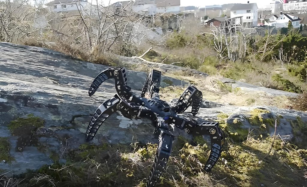
The image above shows the prototype of our hexapod bionic robot during a walking test. The stable tripod gait is evident, with three legs firmly on the ground forming a support triangle while the other three are in the swing phase. The wireless module and IMU are mounted on the central body. During tests, the bionic robot achieved a forward walking speed of approximately 6.45 cm/s. The primary metric for stability was the body acceleration measured by the IMU. The upper computer software plotted real-time acceleration data. A stable walk is characterized by small, bounded oscillations around zero acceleration in the vertical and forward/backward axes. Our tests confirmed that the bionic robot maintained such stable acceleration profiles, indicating successful rejection of disturbances and smooth weight transfer between tripods.
To further analyze the walking performance, we can model the bionic robot’s dynamics simplistically. The force distribution on the stance legs is critical for stability. For a static stance (or quasi-static walking, which is a valid assumption for slow speeds), the condition for stability is that the projection of the center of mass (COM) lies within the support polygon. For a tripod gait, this polygon is a triangle. Let the positions of the three stance feet in the horizontal plane be $\vec{p}_1, \vec{p}_2, \vec{p}_3$. The support triangle $T$ is their convex hull. The COM projection is $\vec{c} = (x_{com}, y_{com})$. Stability requires $\vec{c} \in T$. This can be checked using barycentric coordinates. If the COM is at height $h$ and has total mass $M$, the vertical force $F_i$ on leg $i$ can be approximated (ignoring dynamics) by solving the equilibrium equations:
$$ \sum_{i=1}^{3} F_i = Mg $$
$$ \sum_{i=1}^{3} F_i (\vec{p}_i – \vec{c}) = 0 $$
These forces must be positive for all stance legs. During our bionic robot’s walk, the gait was designed to keep the COM well within the support triangle throughout the cycle. The table below summarizes key performance metrics from the walking experiments.
| Performance Metric | Measured Value | Conditions / Notes |
|---|---|---|
| Forward Speed | 6.45 cm/s | On flat linoleum floor, tripod gait |
| Stride Length | ~40 mm per cycle | Defined as distance body moves per full gait cycle |
| Gait Cycle Frequency | 0.8 Hz | One complete cycle for all legs |
| Peak Vertical Acceleration (RMS) | 0.15 m/s² | Measured by IMU, indicates bounce |
| Power Consumption (Walking) | ~25 Watts | Average during steady walking |
| Turning Capability | Implemented via differential leg speed | Not quantitatively measured in this phase |
While the basic tripod gait provides excellent static stability, the bionic robot’s performance can be enhanced by incorporating dynamic elements and better terrain adaptation. The current open-loop gait generation does not account for uneven ground or slipping. Future iterations of this bionic robot will focus on closed-loop control using additional sensors. A primary upgrade planned is the installation of force-sensitive resistors (FSRs) or contact sensors on each foot tip. This will allow the bionic robot to detect ground contact precisely and adjust leg trajectories in real-time, implementing a reactive walking algorithm. The data from these sensors can be fused with the IMU data to estimate terrain inclination and compensate for shifts in the COM.
Another avenue for improvement is the exploration of other biologically-inspired gaits for the bionic robot. Insects like ants use not only the tripod gait but also wave gaits (where legs move in a sequential wave) for slower, more careful movement, and even transitional gaits for turning. Implementing a gait transition algorithm would make the bionic robot more versatile. Furthermore, optimizing the mechanical structure for weight reduction, perhaps using carbon fiber or advanced polymers, would improve the power-to-weight ratio and allow for longer operation times. The control algorithm could also be extended to include impedance control at the joints, enabling the bionic robot to interact softly with the environment, a key feature for a truly adaptive bionic robot.
In conclusion, the design and implementation of a hexapod bionic robot is a multidisciplinary endeavor that bridges biology, mechanics, and computer science. This project successfully demonstrated a working prototype of a bionic robot that walks stably using a biomimetic leg structure and a tripod gait controlled by a hierarchical software system. The kinematic modeling provided the foundation for motion planning, while the carefully selected hardware components ensured reliable real-time operation. The integration of wireless telemetry allowed for effective monitoring and remote control. The concept of a bionic robot is powerful because it forces us to look to nature for solutions to engineering challenges. This hexapod bionic robot serves as a platform for further research into adaptive locomotion, sensor integration, and autonomous navigation. As we continue to refine this bionic robot, the lessons learned will contribute to the development of more capable and intelligent machines capable of operating in the complex environments that mirror our own world.