
The pursuit of creating machines that emulate the elegance and efficiency of biological organisms has long been a cornerstone of advanced robotics. Among various biomimetic platforms, the multi-legged walking robot, inspired by arthropods, offers distinct advantages over wheeled or tracked systems in unstructured and complex terrains. This article details a thorough exploration into the design, simulation, fabrication, and experimental validation of a fully functional hexapod bionic robot. The development process leverages modern digital tools—specifically, advanced CAD/CAE software for virtual prototyping and 3D printing for physical realization—to create a machine with robust mobility and significant biomimetic appeal.
The fundamental motivation stems from the limitations of conventional locomotion. While wheeled robots excel on prepared surfaces, their performance degrades rapidly on soft, uneven, or obstructed ground. Legged systems, however, can step over gaps, climb obstacles, and maintain stability through adaptable foothold placement. A six-legged (bionic robot) configuration, mirroring insects like cockroaches or beetles, provides an optimal balance between static stability, mechanical complexity, and control manageability. Unlike bipeds or quadrupeds, a hexapod can maintain a statically stable posture (where the center of mass remains within the polygon formed by the supporting feet) even when multiple legs are in motion, simplifying gait generation and control.
Design Principles and Kinematic Analysis
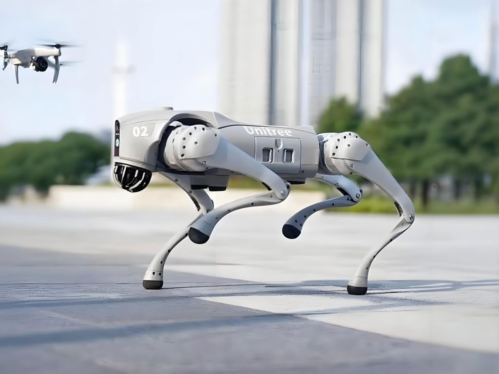
The design of this bionic robot is rooted in a simplified yet effective anatomical model of an insect leg, typically consisting of three primary segments connected by rotary joints. This configuration translates into a robotic leg with three degrees of freedom (3-DOF), often described as having a “hip” joint for forward/backward swing, a “knee” joint for up/down motion, and sometimes a “twist” at the hip for abduction/adduction. For our platform, a 3-DOF design per leg was adopted to ensure sufficient dexterity for navigating varied terrains.
The core body of the bionic robot is a rigid chassis housing the control electronics, battery, and transmission elements. The leg pairs are symmetrically attached. A critical design choice is the gait pattern—the coordinated sequence of leg movements. The most common and inherently stable gait for a hexapod is the alternating tripod gait. In this pattern, the robot’s six legs are divided into two synchronised groups of three (forming a tripod): legs 1, 3, 5 and legs 2, 4, 6. While one tripod is in the swing phase (lifting and moving forward), the other is in the stance phase (pushing backward against the ground to propel the body forward). This gait provides continuous static stability.
The kinematic analysis begins with defining the Denavit-Hartenberg (D-H) parameters for a single leg. This standard convention systematically defines the relationship between consecutive link frames. For a 3-DOF leg with all revolute joints, the parameters can be summarized as follows:
| Joint i | $a_{i-1}$ (Link Length) | $\alpha_{i-1}$ (Link Twist) | $d_i$ (Link Offset) | $\theta_i$ (Joint Angle) |
|---|---|---|---|---|
| 1 (Coxa/Hip) | 0 | 90° | $L_0$ | $\theta_1$ |
| 2 (Femur/Upper Leg) | $L_1$ | 0° | 0 | $\theta_2$ |
| 3 (Tibia/Lower Leg) | $L_2$ | 0° | 0 | $\theta_3$ |
Here, $L_0$, $L_1$, and $L_2$ are the physical lengths of the leg segments. The transformation matrix between frame i-1 and frame i is given by the standard D-H formula:
$$ T_i^{i-1} = \begin{bmatrix}
\cos\theta_i & -\sin\theta_i\cos\alpha_{i-1} & \sin\theta_i\sin\alpha_{i-1} & a_{i-1}\cos\theta_i \\
\sin\theta_i & \cos\theta_i\cos\alpha_{i-1} & -\cos\theta_i\sin\alpha_{i-1} & a_{i-1}\sin\theta_i \\
0 & \sin\alpha_{i-1} & \cos\alpha_{i-1} & d_i \\
0 & 0 & 0 & 1
\end{bmatrix} $$
The overall forward kinematics for the foot position relative to the body frame is obtained by concatenating these transformations:
$$ T_{foot}^{body} = T_0^1 \cdot T_1^2 \cdot T_2^3 $$
The position vector of the foot, $[x, y, z]^T$, is extracted from the last column of $T_{foot}^{body}$. This yields the kinematic equations:
$$ x = L_1 \cos\theta_1 \cos\theta_2 + L_2 \cos\theta_1 \cos(\theta_2 + \theta_3) $$
$$ y = L_1 \sin\theta_1 \cos\theta_2 + L_2 \sin\theta_1 \cos(\theta_2 + \theta_3) $$
$$ z = L_0 + L_1 \sin\theta_2 + L_2 \sin(\theta_2 + \theta_3) $$
Velocity analysis is crucial for smooth motion control. The Jacobian matrix $J(\theta)$ relates the joint angular velocities $\dot{\theta}$ to the Cartesian foot tip velocity $\dot{p}$:
$$ \dot{p} = \begin{bmatrix} v_x \\ v_y \\ v_z \end{bmatrix} = J(\theta) \dot{\theta} $$
For our leg, the Jacobian is a 3×3 matrix derived by differentiating the forward kinematics equations. Its structure ensures we can calculate required joint speeds for a desired foot trajectory during the swing phase. Stability analysis for this bionic robot involves calculating the Center of Mass (CoM) and ensuring its horizontal projection remains within the “support polygon”—the convex hull formed by the points of the feet currently in contact with the ground during the stance phase. For the alternating tripod gait, this polygon is always a triangle, providing inherent static stability if the CoM projection is properly managed.
Motion Modeling and Simulation
Before physical assembly, a comprehensive virtual prototype was developed using Siemens NX 10.0. This digital twin allowed for rigorous motion simulation and optimization, significantly reducing development time and cost. The process followed a systematic workflow:
1. 3D Modeling: Each mechanical component—chassis, servo brackets, leg links, gears, and shafts—was meticulously modeled using parametric features, ensuring dimensional accuracy and assemblability.
2. Assembly: Components were virtually assembled with appropriate constraints (mates), replicating the final mechanical configuration of the bionic robot.
3. Motion Simulation Setup: Within the Motion Simulation module, the model was prepared for dynamics analysis.
• Link Creation: Each rigid part was defined as a “Link” (e.g., L001: Chassis, L002: Coxa Link, etc.).
• Joint Creation: Kinematic joints were applied between links. Servo outputs were modeled as revolute joints with motor drivers. Gear contacts were defined as gear couplings or 3D contact constraints.
• Drive Definition: A constant rotational speed driver (e.g., 100 deg/s) was applied to the primary drive servo’s joint to initiate movement.
• Solution Creation: A solver scheme was configured with parameters such as analysis time (e.g., 10 seconds) and number of steps (e.g., 500). A marker was placed on one foot tip to trace its trajectory.
4. Simulation and Analysis: The solver calculated the system’s motion over time. Key results, such as the displacement, velocity, and acceleration of the marked foot point, were plotted. The foot trajectory, a critical characteristic of the bionic robot‘s gait, was visualized. The smoothness of the velocity and acceleration curves indicated the dynamic performance and helped identify potential issues like jerky motion or excessive inertial forces.
The simulation provided quantitative data essential for refinement. For instance, the foot trajectory during a full step cycle can be characterized by key parameters:
| Trajectory Phase | Description | Key Metric (Example Value) |
|---|---|---|
| Swing (Lift-off) | Foot lifts vertically to clear ground. | Max height: 25 mm |
| Swing (Forward) | Foot moves forward relative to body. | Stride length: 80 mm |
| Swing (Touch-down) | Foot descends vertically to ground. | Impact velocity: < 0.1 m/s |
| Stance (Power stroke) | Foot pushes backward, propelling body. | Backward displacement: 80 mm |
The velocity $v(t)$ and acceleration $a(t)$ profiles of the foot marker, derived from the simulation, can be approximated by sinusoidal or polynomial functions to inform control algorithms. For example, a cycloidal trajectory is often used for smooth motion:
$$ s(t) = S \left( \frac{t}{T} – \frac{1}{2\pi} \sin\left(\frac{2\pi t}{T}\right) \right) $$
where $s(t)$ is the position along the path, $S$ is the total stroke length, $T$ is the swing phase duration, and $t$ is time. The corresponding velocity is:
$$ v(t) = \frac{S}{T} \left(1 – \cos\left(\frac{2\pi t}{T}\right)\right) $$
This ensures zero velocity at the start and end of the swing phase, minimizing impact.
Control System Architecture
The intelligence of the bionic robot resides in its electronic control system, which translates high-level commands into precise servo movements. The architecture is hierarchical.
Hardware Layer: The core is a microcontroller (e.g., Arduino Mega, STM32, or ESP32) chosen for its sufficient number of Pulse Width Modulation (PWM) outputs to control all 18 servos (3 per leg x 6 legs). It receives commands from a user interface (like a Bluetooth app or a radio controller) and reads data from optional sensors (Inertial Measurement Units – IMUs, distance sensors). A dedicated servo driver board or a power distribution board with adequate current rating is essential to handle the peak current draw of multiple servos moving simultaneously.
Software Layer – Gait Engine: The core algorithm is the gait generator. For the alternating tripod gait, it manages two state machines for the two leg groups. Based on a timer or a commanded speed, it cycles through the swing and stance phases. It calculates the desired foot trajectory in Cartesian space (body coordinates) for the swing legs using predefined path equations (like the cycloidal one mentioned). For the stance legs, it calculates a simple backward linear motion relative to the body to create forward propulsion.
Software Layer – Inverse Kinematics (IK) Solver: This is the computational heart. For each leg in motion, the desired foot position $(x_d, y_d, z_d)$ is fed into the IK solver, which calculates the required joint angles $(\theta_1, \theta_2, \theta_3)$. For a 3-DOF leg, this often involves geometric or algebraic methods. One common solution involves calculating $\theta_1$ first using the projected point on the ground plane:
$$ \theta_1 = \arctan2(y_d, x_d) $$
Then, the distance from the hip joint to the foot projection on the leg plane, $r = \sqrt{x_d^2 + y_d^2}$, and the height difference are used. Defining $D = \frac{r^2 + (z_d – L_0)^2 – L_1^2 – L_2^2}{2 L_1 L_2}$, we can solve for $\theta_3$ and $\theta_2$:
$$ \theta_3 = \arctan2(\pm\sqrt{1-D^2}, D) $$
$$ \theta_2 = \arctan2(z_d – L_0, r) – \arctan2(L_2 \sin\theta_3, L_1 + L_2 \cos\theta_3) $$
The choice of sign for $\theta_3$ corresponds to different elbow configurations (e.g., “elbow up” vs “elbow down”).
Motion Planning & Navigation: Higher-level behaviors can be implemented. Turning is achieved by applying a scaling factor to the stride length of legs on one side relative to the other. Omni-directional movement can be realized by superimposing a lateral component on the foot trajectory during the swing phase. The controller can be represented by a simplified block diagram and equation:
$$ \Theta_{cmd}(t) = IK \left( GaitGenerator(v, \omega, t) \right) + P(\Theta_{desired} – \Theta_{feedback}) $$
Where $v$ is forward speed, $\omega$ is turning rate, and $P$ is a proportional correction term from optional joint feedback.
Structural Design and 3D Printing Fabrication
The transition from digital model to physical bionic robot was achieved using Fused Deposition Modeling (FDM) 3D printing. This additive manufacturing technique offers unparalleled design freedom, allowing for the creation of complex, lightweight, and integrated geometries that would be difficult or expensive to produce using traditional methods.
Material Selection: Polylactic Acid (PLA) was chosen for the initial prototypes due to its ease of printing, good stiffness, and low cost. For more durable and demanding versions, Acrylonitrile Butadiene Styrene (ABS) or Polycarbonate (PC) blends can be used, offering higher impact resistance and thermal stability. Key material properties considered include tensile strength, layer adhesion, and fatigue resistance under cyclic loading from leg movements.
Component Design for Additive Manufacturing: Parts were optimized for 3D printing. This involved:
• Designing appropriate wall thicknesses (typically 2-4 mm) for strength without excessive weight.
• Incorporating internal ribbing or lattice structures in large flat areas like the chassis to prevent warping and increase rigidity.
• Minimizing the need for support material through intelligent orientation and self-supporting angles (typically > 45°).
• Designing integrated fastener features like captive nut slots or heat-set inserts for robust assembly.
Printing and Post-Processing: The components were sliced using software (e.g., Ultimaker Cura, PrusaSlicer) with optimized parameters for layer height (0.2 mm for strength, 0.15 mm for detail), infill density (20-40% for most parts, higher for critical joints), and print speed. After printing, support material was removed, and parts were cleaned. Critical bearing and shaft holes were sometimes drilled or reamed to ensure precise dimensions. Finally, components were assembled using screws, bearings, and the purchased electronic and actuation components (servos, controller, battery).
A summary of the primary structural components is as follows:
| Component | Primary Function | Key Design Features | Print Material/Notes |
|---|---|---|---|
| Main Chassis/Body | Houses electronics, provides mounting for leg pairs. | Internal ribbing, cable routing channels, ventilation holes, mounting bosses. | PLA/ABS, 30% infill |
| Coxa (Hip) Bracket | Attaches leg to body, houses 1st (yaw) servo. | Strong servo horn attachment, bearing seat for robustness. | PLA, 40% infill |
| Femur (Upper Leg) Link | Connects coxa to tibia, houses 2nd (pitch) servo. | Lightweight truss design, secure servo pockets. | PLA, 25% infill |
| Tibia (Lower Leg) Link | Terminates at foot, houses 3rd (pitch) servo or acts as passive link. | Tapered for weight saving, textured foot tip for grip. | PLA, 25% infill |
| Servo Horns & Couplers | Transmit torque from servo to link. | Precise spline or D-shape fit, grub screw seats. | PLA, 80% infill for strength |
Experimental Validation and Performance Analysis
The finalized physical prototype of the bionic robot underwent a series of experiments to validate the simulation models and assess real-world performance.
Test Setup: Experiments were conducted on various surfaces: smooth floor, low-pile carpet, and an outdoor grassy area. The robot was operated via remote control, executing forward/backward motion, in-place turns, and later, pre-programmed autonomous sequences. Data was collected qualitatively through observation and video recording, and quantitatively by measuring traverse time over a fixed distance, observing stability during turning, and noting any mechanical failures.
Mobility and Gait Performance: The bionic robot successfully demonstrated stable locomotion using the alternating tripod gait. Its speed on flat ground was primarily limited by the servo speed and stride length. The turning radius was adjustable based on the differential drive logic applied to the leg pairs. The robot showed a clear advantage on soft grass compared to a hypothetical small wheeled robot, as its feet did not sink in significantly and could step over minor irregularities.
Stability Assessment: The static stability inherent to the tripod gait was confirmed. The robot could come to a complete halt at any point in the gait cycle without falling. Dynamic stability during continuous motion was good, though rapid direction changes could induce noticeable body rocking, highlighting the need for future integration of an IMU and active body-leveling control—an advanced step for this class of bionic robot.
Power and Endurance: Current draw was monitored. Peak current occurred when all servos in the stance phase were under load simultaneously. A significant finding was the importance of a well-balanced power management system to prevent brownouts in the microcontroller during high-torque maneuvers.
A summary of key experimental observations is tabulated below:
| Performance Metric | Test Condition (Flat Indoor) | Result & Observation |
|---|---|---|
| Forward Speed | Moderate servo speed setting | ~8-10 cm/s. Limited by servo rotation rate and stride geometry. |
| Turning Agility | In-place (“spot”) turn | ~20-30 degrees/second. Smooth and stable. |
| Stair/Obstacle Climbing | 10 mm tall wooden block | Successful. Swing leg trajectory cleared the obstacle. |
| Terrain Adaptability | Transition from tile to carpet | No significant performance degradation. Gait remained stable. |
| Continuous Operation Time | With 2000mAh LiPo battery | ~45-60 minutes of intermittent operation. |
The experiments validated the core design and confirmed that the integration of virtual prototyping and additive manufacturing is a highly effective pipeline for developing functional legged bionic robot platforms. The demonstrated mobility and stability form a solid foundation for future enhancements.
Conclusion and Future Trajectory
This comprehensive project has successfully detailed the complete lifecycle of a hexapod bionic robot, from conceptual biomimetic principles and detailed kinematic modeling through digital simulation and additive manufacturing to physical experimentation. The alternating tripod gait proved to be a robust and easily implementable control scheme, providing the machine with reliable static stability and adequate mobility across different terrains. The use of UG NX for virtual prototyping allowed for the prediction and optimization of motion characteristics, while 3D printing enabled the rapid, cost-effective realization of a complex mechanical structure that would be challenging to fabricate otherwise.
The finished bionic robot serves as a potent platform for research and development in bio-inspired robotics. Several compelling directions for future work immediately present themselves. Firstly, the sensory apparatus can be greatly expanded. Integrating an Inertial Measurement Unit (IMU) would allow for active body posture stabilization and more sophisticated dynamic gait control. Adding distance sensors (ultrasonic, infrared, or LiDAR) or cameras would enable autonomous navigation and obstacle avoidance, moving the platform from tele-operation to true autonomy.
Secondly, the mechanical design can be evolved. Employing composite materials or advanced printing polymers like nylon or PETG-CF could reduce weight while increasing strength. Implementing more advanced joint designs with series elastic actuators or even variable stiffness mechanisms could improve energy efficiency and impact tolerance, making the bionic robot more robust and lifelike in its movement. Finally, the control algorithms can graduate from fixed, pre-programmed gaits to adaptive ones. Machine learning techniques, such as reinforcement learning, could be employed to allow the robot to learn optimal gaits for specific terrains or to recover from slips and falls autonomously.
In conclusion, the field of legged bionic robot development is richly interdisciplinary, merging biology, mechanical engineering, electronics, and computer science. The platform described herein acts as a foundational step, demonstrating the viability and excitement of creating machines that walk as living creatures do. The iterative cycle of design, simulation, fabrication, and test remains the cornerstone of innovation in this domain, promising ever more capable and versatile walking machines for exploration, assistance, and discovery in the years to come.