
Industrial robot absolute positioning accuracy is one of the decisive factors limiting the deployment of robotic systems in high-value manufacturing tasks such as welding, precision grinding, drilling, and component assembly. In these operations, even sub-millimeter deviations at the end-effector can propagate into unacceptable geometric nonconformity, degraded surface integrity, or assembly failure. When I analyze the error budget of a serial industrial robot, I find that two contributions dominate: geometric errors generated by manufacturing and assembly imperfections, and flexibility-induced errors caused by payload variation and the associated joint torque redistribution. These two contributions have fundamentally different physical origins, yet they appear jointly in the measured pose error and therefore must be modeled in a unified manner. In this work, I propose an adaptive dual-branch physics-informed neural network with a constraint weight adapter, abbreviated as PC-DBPINN-CWA, to predict and compensate the pose error of an industrial robot under variable payload conditions. The core idea is to separate the two physical mechanisms inside the network architecture and then re-couple them through a supervised additive fusion, while embedding explicit physical constraints into the training objective so that the learned mapping remains physically admissible outside the training distribution.
The remainder of this article is organized as follows. I first describe the kinematic and error description of the industrial robot, including the modified Denavit–Hartenberg formulation, the geometric error model, and the payload-induced flexibility error model. Then I present the dual-branch physics-informed architecture and the associated physics-based loss terms. After that, I introduce the residual-feedback constraint weight adapter and derive the adaptive loss balancing rule. Finally, I report the experimental validation on a six-degree-of-freedom industrial robot, including ablation studies, comparisons with published baselines, and online compensation results obtained under unseen payloads.
Kinematic Modeling and Error Description of the Industrial Robot
I build the forward kinematic model of the industrial robot using the modified Denavit–Hartenberg convention, because it avoids the singularity that occurs in the standard convention when two consecutive joint axes are parallel. For two adjacent link frames, the homogeneous transformation matrix is written as
$${}^{i-1}T_i = \mathrm{Rot}(z,\theta_i)\,\mathrm{Trans}(z,d_i)\,\mathrm{Trans}(x,a_i)\,\mathrm{Rot}(x,\alpha_i)\,\mathrm{Rot}(y,\beta_i)$$
where $a_i$ is the link length, $\alpha_i$ is the link twist, $d_i$ is the link offset, $\theta_i$ is the joint angle, and $\beta_i$ is the additional rotation about the $y$-axis that is required only when two consecutive joint axes are parallel. For a six-axis industrial robot with parallel second and third axes, all remaining $\beta_i$ values vanish. The forward kinematics of the industrial robot is obtained by multiplying the six link transformations,
$${}^{0}T_6 = \prod_{i=1}^{6}{}^{i-1}T_i = \begin{bmatrix} R & P \\ 0 & 1 \end{bmatrix}$$
where $R$ is the orientation matrix of the end-effector and $P = [X, Y, Z]^T$ is the position vector of the end-effector expressed in the base frame. I parameterize the orientation by the Euler angles $[A, B, C]^T$ through the relations
$$A = \arctan2(r_{32}, r_{33}), \qquad B = \arctan2\!\left(-r_{31}, \sqrt{r_{11}^{2} + r_{21}^{2}}\right), \qquad C = \arctan2(r_{21}, r_{11})$$
so that the theoretical pose of the industrial robot is represented by the six-dimensional vector $[X, Y, Z, A, B, C]^T$. This theoretical pose forms the geometric input of the first branch of my network, and the joint angles extracted from the controller form the differentiation variables used by the geometric smoothness constraint.
I assume that the total pose error of the industrial robot can be decomposed into a geometric part and a flexibility part in an additive manner. This assumption is justified for quasi-static operation and small deformations, where the two mechanisms act independently to first order. Therefore,
$$\delta e = \delta e_g + \delta e_f$$
where $\delta e_g$ is the geometric error component and $\delta e_f$ is the flexibility error component. Both components are six-dimensional vectors containing three position errors and three orientation errors.
Geometric Error of the Industrial Robot
Geometric errors of the industrial robot arise from manufacturing tolerances, assembly deviations, and wear of the structural components. If I denote the nominal link parameters by $\theta_i, d_i, a_i, \alpha_i, \beta_i$ and their actual values by $\theta_i + \Delta\theta_i$, $d_i + \Delta d_i$, $a_i + \Delta a_i$, $\alpha_i + \Delta\alpha_i$, and $\beta_i + \Delta\beta_i$, the actual transformation matrix of each link becomes a perturbed version of the nominal one. The deviation between the actual and theoretical end-effector transforms is
$$\delta T_g = T_{\text{actual}} – T_{\text{theory}}$$
and the resulting geometric error vector of the industrial robot is
$$\delta e_g = \begin{bmatrix} \delta X_g & \delta Y_g & \delta Z_g & \delta A_g & \delta B_g & \delta C_g \end{bmatrix}^{T}$$
where the first three components describe the position error and the last three components describe the orientation error. It is well known that geometric errors evolve smoothly with the robot configuration, because they are determined by fixed structural parameters rather than by external loads. I exploit this property explicitly by embedding a geometric smoothness constraint into the training of the geometric branch, which prevents the network from learning nonphysical high-frequency fluctuations.
Payload-Induced Flexibility Error of the Industrial Robot
When a payload is mounted on the end-effector of the industrial robot, the gravity load and the inertial load change the torque state of each joint, producing elastic deformation in the drivetrains, gearboxes, and links. I model each joint as a linear torsional spring, which is a widely adopted approximation for the quasi-static regime. The equivalent joint torque produced by an external wrench is obtained from the static equilibrium condition,
$$\tau(\theta) = J^{T}(\theta) F$$
where $J(\theta)$ is the geometric Jacobian of the industrial robot and $F$ is the external force and torque vector acting on the end-effector. The elastic deformation of the joints follows the linear torsional spring model,
$$\Delta\theta = C\,\tau(\theta), \qquad C = \mathrm{diag}(c_1, c_2, c_3, c_4, c_5, c_6)$$
where $C$ is the joint compliance matrix and $c_1$ through $c_6$ are the compliance coefficients of the six joints. The joint deformation is mapped to the end-effector through the differential kinematic relation,
$$\delta e_f = J(\theta)\,\Delta\theta = J(\theta)\,C\,J^{T}(\theta)\,F$$
which is the comprehensive flexibility deformation model of the industrial robot. The resulting flexibility error vector is
$$\delta e_f = \begin{bmatrix} \delta X_f & \delta Y_f & \delta Z_f & \delta A_f & \delta B_f & \delta C_f \end{bmatrix}^{T}$$
Because the flexibility error of the industrial robot depends on the payload mass, the payload center of mass, and the motion state, I feed these quantities into the second branch of the network together with the instantaneous velocity and acceleration statistics of the joints. In this way, the flexibility branch learns a mapping that is conditioned on the actual loading condition rather than on the geometric configuration alone.
Dual-Branch Physics-Informed Neural Network Architecture
Physics-informed neural networks provide a principled way to combine data-driven learning with known physical laws. Instead of learning an arbitrary function from inputs to outputs, the network is trained to minimize a composite objective that contains both a data-fitting term and one or more physical residual terms. In the context of industrial robot error modeling, this is particularly valuable because the number of measured poses is limited, payload conditions are only partially sampled, and a purely data-driven model can easily produce predictions that violate the known mechanics of the industrial robot.
I construct a dual-branch architecture in which the geometric error and the flexibility error are predicted by two separate sub-networks. The two branches share no weights, because the two error mechanisms have different input spaces and different physical behaviors. The geometric branch takes the theoretical pose of the industrial robot as input and predicts the six-dimensional geometric error. The flexibility branch takes the payload parameters and the motion-state descriptors as input and predicts the six-dimensional flexibility error. The two predictions are then summed to form the total pose error,
$$\delta \hat{e} = \delta \hat{e}_g + \delta \hat{e}_f$$
This additive fusion is consistent with the first-order superposition assumption stated earlier, and it allows each branch to be regularized by physical constraints that are specific to its own mechanism.
Geometric Error Sub-Network
The geometric branch receives the theoretical pose of the industrial robot,
$$x_g = \begin{bmatrix} X & Y & Z & A & B & C \end{bmatrix}^{T} \in \mathbb{R}^{6}$$
which is obtained from the nominal forward kinematic model. This input vector describes the configuration of the industrial robot in task space and is independent of the payload. The sub-network $\mathcal{G}$ is a fully connected multilayer perceptron with three hidden layers and rectified linear unit activations, and it produces the geometric error estimate
$$\delta \hat{e}_g = \mathcal{G}(x_g; \xi_g)$$
where $\xi_g$ denotes the trainable parameters of the geometric branch. I deliberately keep this branch relatively compact, because the geometric error of an industrial robot is a smooth function of the configuration and does not require a very deep representation. The smoothness constraint described in the next section further restricts the hypothesis space and improves extrapolation to configurations that were not visited during data collection.
Flexibility Error Sub-Network
The flexibility branch receives a six-dimensional descriptor that combines the payload properties with the motion-state statistics,
$$x_f = \begin{bmatrix} x_{\text{cog}} & y_{\text{cog}} & z_{\text{cog}} & m & \bar{q} & \bar{\ddot{q}} \end{bmatrix}^{T}$$
where $[x_{\text{cog}}, y_{\text{cog}}, z_{\text{cog}}]$ is the payload center of mass, $m$ is the payload mass, and $\bar{q}$ and $\bar{\ddot{q}}$ are the mean absolute joint speed and the mean absolute joint acceleration of the industrial robot. Because the controller only provides discrete joint position samples at a fixed rate, I reconstruct the velocity and acceleration fields by central finite differences,
$$\dot{q}_i(t_k) \approx \frac{q_i(t_{k+1}) – q_i(t_{k-1})}{2\Delta t}, \qquad \ddot{q}_i(t_k) \approx \frac{q_i(t_{k+1}) – 2q_i(t_k) + q_i(t_{k-1})}{\Delta t^{2}}$$
and then apply spatial mean pooling over the six joints,
$$\bar{q} = \frac{1}{6}\sum_{i=1}^{6} \left| \dot{q}_i \right|, \qquad \bar{\ddot{q}} = \frac{1}{6}\sum_{i=1}^{6} \left| \ddot{q}_i \right|$$
The flexibility sub-network $\mathcal{F}$ is also a fully connected multilayer perceptron, and it produces the flexibility error estimate
$$\delta \hat{e}_f = \mathcal{F}(x_f; \xi_f)$$
where $\xi_f$ denotes the trainable parameters of the flexibility branch. The separation of the two branches is the key architectural choice of my method, because it allows the geometric smoothness constraint to act only on the geometric branch and the force–deformation constraints to act only on the flexibility branch. If a single monolithic network were used, these constraints would interfere with each other and the optimization would become unnecessarily difficult.
| Branch | Input vector | Physical meaning | Output |
|---|---|---|---|
| Geometric sub-network | $[X, Y, Z, A, B, C]^T$ | Configuration-dependent geometric deviation | $\delta \hat{e}_g \in \mathbb{R}^6$ |
| Flexibility sub-network | $[x_{\text{cog}}, y_{\text{cog}}, z_{\text{cog}}, m, \bar{q}, \bar{\ddot{q}}]^T$ | Payload and motion-dependent elastic deformation | $\delta \hat{e}_f \in \mathbb{R}^6$ |
| Fusion | $\delta \hat{e}_g + \delta \hat{e}_f$ | Superposition of the two independent error mechanisms | $\delta \hat{e} \in \mathbb{R}^6$ |
Physics-Based Loss Function Design
The data-fitting loss alone cannot guarantee that the predictions of the industrial robot error model remain physically meaningful outside the sampled payload range. I therefore introduce three physics-based loss terms, two of which act on the flexibility branch and one of which acts on the geometric branch. The overall training objective is a weighted sum of the data terms and the physical residual terms, and the weights are adapted during training by the constraint weight adapter.
Geometric Smoothness Constraint
The geometric error of the industrial robot is caused by fixed structural parameter deviations, and therefore it varies continuously and smoothly with the joint configuration. A small change in a joint angle should produce only a small change in the geometric error. I enforce this property by penalizing the sensitivity of the predicted geometric error with respect to each joint angle,
$$\mathcal{L}_{\text{geo}} = \frac{1}{N}\sum_{n=1}^{N} \frac{1}{6}\sum_{i=1}^{6} \left\| \frac{\partial \delta \hat{e}_g^{(n)}}{\partial \theta_i} \right\|^{2}$$
where $N$ is the batch size and $\theta_i$ is the $i$-th joint angle of the industrial robot. The partial derivatives are computed by automatic differentiation, so no additional measurement or finite-difference approximation is required. This constraint suppresses nonphysical oscillations and improves the local stability of the geometric prediction, which is especially important near the boundaries of the workspace.
Force–Deformation Direction Consistency Constraint
Under an external load, the end-effector of the industrial robot deforms along a direction that is determined by the pose-dependent Cartesian compliance. I compute the Cartesian compliance matrix from the Jacobian and the joint compliance matrix,
$$C_{\text{cart}}(\theta) = J(\theta)\,C\,J^{T}(\theta)$$
and the theoretical deformation direction is obtained by normalizing the compliance-weighted external force,
$$d_{\text{theory}} = \frac{C_{\text{cart}}(\theta) F}{\left\| C_{\text{cart}}(\theta) F \right\|}$$
The predicted deformation direction is obtained from the position part of the predicted flexibility error,
$$d_{\text{pred}} = \frac{\delta \hat{p}_f}{\left\| \delta \hat{p}_f \right\|}, \qquad \delta \hat{p}_f = \begin{bmatrix} \delta \hat{X}_f & \delta \hat{Y}_f & \delta \hat{Z}_f \end{bmatrix}^{T}$$
I then require the two directions to be aligned, which is expressed by the squared deviation of their inner product from unity,
$$\mathcal{L}_{\text{direction}} = \frac{1}{N}\sum_{n=1}^{N} \left[ 1 – \left( d_{\text{pred}}^{(n)} \cdot d_{\text{theory}}^{(n)} \right) \right]^{2}$$
This constraint is particularly effective at medium and high payloads, because it forces the flexibility branch to respect the directional anisotropy of the industrial robot stiffness rather than fitting an arbitrary vector field.
Energy Conservation Constraint
According to the principle of virtual work, the work done by the external load during the elastic deformation must equal the strain energy stored in the structure. I write the external work as
$$W_{\text{external}} = F^{T} \delta \hat{p}_f$$
and the stored strain energy as
$$U_{\text{strain}} = \frac{1}{2} \delta \hat{p}_f^{T} K \delta \hat{p}_f, \qquad K = \left( J(\theta)\,C\,J^{T}(\theta) \right)^{-1}$$
The energy conservation residual is then penalized as
$$\mathcal{L}_{\text{energy}} = \frac{1}{N}\sum_{n=1}^{N} \left| U_{\text{strain}}^{(n)} – W_{\text{external}}^{(n)} \right|$$
This term bounds the magnitude of the predicted deformation and prevents the flexibility branch from producing unrealistically large displacements, which is a common failure mode of purely data-driven models when the payload is outside the training range.
| Constraint | Branch | Mathematical form | Physical role |
|---|---|---|---|
| Geometric smoothness | Geometric | $\mathcal{L}_{\text{geo}}$ | Suppresses nonphysical fluctuations with respect to joint angles |
| Force–deformation direction | Flexibility | $\mathcal{L}_{\text{direction}}$ | Aligns predicted deformation with the compliance-weighted load direction |
| Energy conservation | Flexibility | $\mathcal{L}_{\text{energy}}$ | Enforces the balance between external work and stored strain energy |
Composite Loss and Adaptive Constraint Weight Adapter
The data loss of each branch is defined as the mean squared error between the predicted and measured error components,
$$\mathcal{L}_{\text{data}}^{g} = \frac{1}{N}\sum_{n=1}^{N} \frac{1}{2}\left\| y_g^{(n)} – \hat{y}_g^{(n)} \right\|^{2}, \qquad \mathcal{L}_{\text{data}}^{f} = \frac{1}{N}\sum_{n=1}^{N} \frac{1}{2}\left\| y_f^{(n)} – \hat{y}_f^{(n)} \right\|^{2}$$
The branch-level losses are then written as
$$\mathcal{L}_g = \lambda_{g,1}\mathcal{L}_{\text{data}}^{g} + \lambda_{g,2}\mathcal{L}_{\text{geo}}$$
$$\mathcal{L}_f = \lambda_{f,1}\mathcal{L}_{\text{data}}^{f} + \lambda_{f,2}\mathcal{L}_{\text{direction}} + \lambda_{f,3}\mathcal{L}_{\text{energy}}$$
Rather than selecting the weights $\lambda$ manually, I introduce a learnable uncertainty parameter $\sigma_a$ for each loss term and formulate the adapter loss as
$$\mathcal{L}_{\text{CWA}} = \sum_{a} \left( \frac{1}{2\sigma_a^{2}} \mathcal{L}_a + \log \sigma_a \right)$$
so that the effective weight of each term becomes
$$\lambda_a = \frac{1}{\sigma_a^{2}}$$
The logarithmic term prevents the uncertainty parameters from diverging to extreme values and therefore stabilizes the optimization. The adapter behaves in an intuitive way. When a physical residual is large and noisy at the beginning of training, the corresponding $\sigma_a$ increases and the effective weight decreases, so the constraint does not overwhelm the data term. As the residual decreases and the constraint becomes learnable, $\sigma_a$ shrinks and the effective weight grows, so the physical constraint dominates the late stage of training. This dynamic balancing is the reason why the industrial robot error model remains accurate across the entire payload range.
Experimental Setup and Data Acquisition
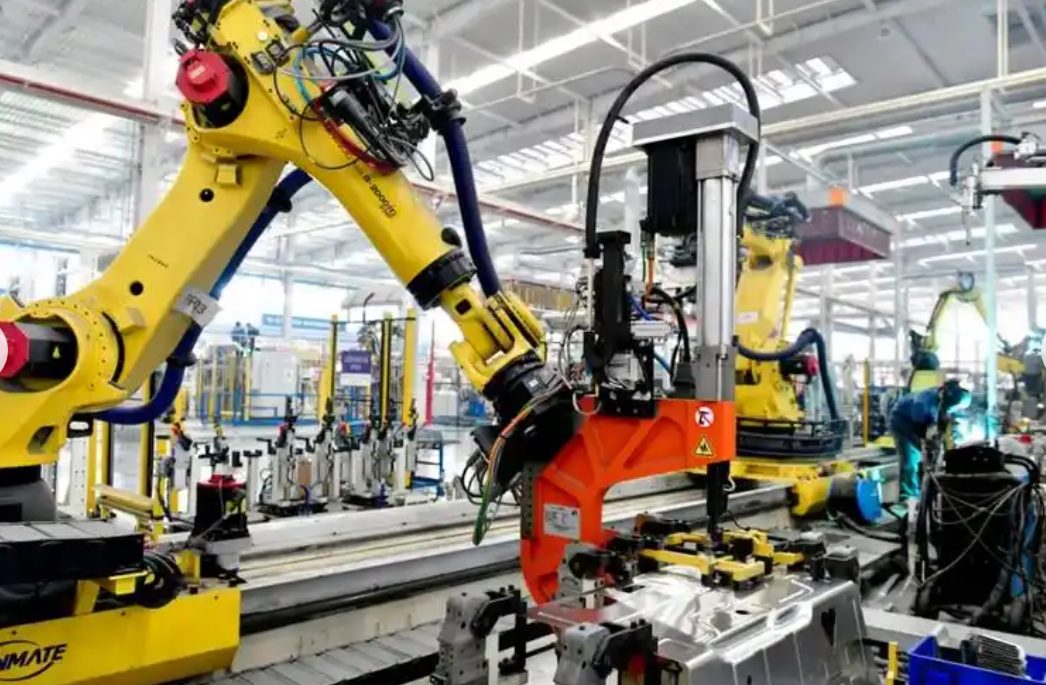
I validate the proposed method on a six-degree-of-freedom industrial robot with a rated payload of sixteen kilograms. The end-effector pose is measured by a laser tracker with a nominal accuracy of $0.015\ \text{mm} + 0.006\ \text{mm/m}$ together with a reflector target, and an online communication and control software package exchanges motion commands and state data with the robot controller over TCP/IP. The measurement volume is a cube with an edge length of five hundred millimeters, discretized with a grid spacing of fifty millimeters, which yields eleven points per axis and a total of one thousand three hundred thirty-one measurement points per payload condition. Four payload conditions are used, namely no payload, seven kilograms, eleven kilograms, and fifteen kilograms, giving a total of five thousand three hundred twenty-four measured poses. The data set is divided into a training set and a validation set with a ratio of eight to two, and the industrial robot moves at fifty percent of its rated speed during the entire acquisition.
The data collected under the no-payload condition mainly reflects the geometric error of the industrial robot, because the payload-induced deformation is absent. The data collected under the loaded conditions contain both the geometric error and the flexibility error, and they are used to supervise the flexibility branch after the geometric contribution has been separated. I observe that the axial positioning errors grow in magnitude and dispersion as the payload increases. For the fifteen-kilogram condition, the mean error along the X direction shifts from $0.155\ \text{mm}$ to $-0.077\ \text{mm}$ and the standard deviation increases to $0.628\ \text{mm}$. The Z direction is dominated by gravity, and its mean shifts from $0.215\ \text{mm}$ to $-0.734\ \text{mm}$, which indicates a downward sag of the end-effector. The Y direction fluctuates around zero but its range increases to $0.50\ \text{mm}$. The mean absolute positioning error grows from $0.308\ \text{mm}$ under no payload to $0.889\ \text{mm}$ under fifteen kilograms, and the maximum absolute error reaches $1.457\ \text{mm}$. These statistics confirm that payload variation is a first-order contributor to the pose error of the industrial robot and that a purely geometric calibration cannot compensate it.
Ablation Study of the Proposed Industrial Robot Error Model
I conduct an ablation study to quantify the contribution of each architectural and physical component. The variants include the plain physics-informed network, the dual-branch network without physical constraints, the dual-branch network with a single physical constraint, the dual-branch network with all constraints and fixed weights, and the full model with the adaptive constraint weight adapter. The root mean square error of the position and orientation predictions is reported for each payload condition.
| Model | Payload | Position RMSE (mm) | Orientation RMSE (deg) |
|---|---|---|---|
| PINN | No payload | 0.08009 | 0.06585 |
| 7 kg | 0.24126 | 0.12321 | |
| 11 kg | 0.31173 | 0.13710 | |
| 15 kg | 0.38162 | 0.14859 | |
| DBPINN | No payload | 0.07407 | 0.05278 |
| 7 kg | 0.20301 | 0.09957 | |
| 11 kg | 0.27946 | 0.11058 | |
| 15 kg | 0.36128 | 0.12087 | |
| PC-DBPINN + geometric smoothness | No payload | 0.05821 | 0.04512 |
| 7 kg | 0.18235 | 0.09345 | |
| 11 kg | 0.27185 | 0.11876 | |
| 15 kg | 0.34267 | 0.12984 | |
| PC-DBPINN + direction consistency | No payload | 0.06412 | 0.04893 |
| 7 kg | 0.17025 | 0.08537 | |
| 11 kg | 0.23874 | 0.10625 | |
| 15 kg | 0.29816 | 0.10842 | |
| PC-DBPINN + energy conservation | No payload | 0.06685 | 0.05021 |
| 7 kg | 0.17654 | 0.08972 | |
| 11 kg | 0.23147 | 0.09854 | |
| 15 kg | 0.27639 | 0.10411 | |
| PC-DBPINN + all constraints (fixed weights) | No payload | 0.06267 | 0.04634 |
| 7 kg | 0.19266 | 0.09167 | |
| 11 kg | 0.24768 | 0.11034 | |
| 15 kg | 0.30647 | 0.11091 | |
| PC-DBPINN-CWA (proposed) | No payload | 0.05339 | 0.04390 |
| 7 kg | 0.16084 | 0.08214 | |
| 11 kg | 0.20782 | 0.09133 | |
| 15 kg | 0.25441 | 0.09687 |
The comparison between the plain physics-informed network and the dual-branch network confirms that separating the two error mechanisms is beneficial. At fifteen kilograms, the position RMSE decreases from $0.38162\ \text{mm}$ to $0.36128\ \text{mm}$, a reduction of $5.33\%$, while the orientation RMSE decreases from $0.14859$ degrees to $0.12087$ degrees, a reduction of $18.65\%$. The improvement is not uniform across payloads, because the geometric branch benefits most from the no-payload data while the flexibility branch benefits from the loaded data. This is precisely the behavior that I expect from a physically separated architecture.
Adding a single physical constraint produces a constraint-specific improvement pattern. The geometric smoothness constraint gives the best no-payload accuracy, with a position RMSE of $0.05821\ \text{mm}$, but its advantage shrinks as the payload grows and reaches $0.34267\ \text{mm}$ at fifteen kilograms. The direction consistency constraint performs better at medium and high payloads, reaching $0.23874\ \text{mm}$ at eleven kilograms and $0.29816\ \text{mm}$ at fifteen kilograms. The energy conservation constraint gives the best single-constraint performance at the maximum payload, namely $0.27639\ \text{mm}$, which shows that bounding the deformation magnitude is an effective way to stabilize the industrial robot error model under heavy loading. When all constraints are combined with fixed weights, the performance is better than the unconstrained dual-branch model but still inferior to the adaptive variant, which demonstrates that the relative weighting of the constraints matters as much as their presence.
The full model with the constraint weight adapter achieves the best accuracy in every test case. Compared with the fixed-weight variant, the adaptive model reduces the no-payload position RMSE from $0.06267\ \text{mm}$ to $0.05339\ \text{mm}$, a reduction of $14.81\%$, and reduces the seven-kilogram position RMSE from $0.19266\ \text{mm}$ to $0.16084\ \text{mm}$, a reduction of $16.51\%$. Relative to the plain physics-informed network at fifteen kilograms, the proposed model lowers the position RMSE from $0.38162\ \text{mm}$ to $0.25441\ \text{mm}$, a reduction of $33.33\%$, and lowers the orientation RMSE from $0.14859$ degrees to $0.09687$ degrees, a reduction of $34.81\%$. I attribute this consistent gain to the fact that the adapter resolves the scale mismatch between the data loss and the physical residuals automatically, instead of relying on a hand-tuned schedule.
The evolution of the loss weights during training confirms this interpretation. In the geometric branch, the data loss dominates the early stage and the smoothness weight remains low. As training proceeds, the smoothness weight rises and stabilizes between approximately $2.0$ and $2.8$, while the data weight falls to approximately $0.8$ to $1.0$. In the flexibility branch, the direction consistency and energy conservation weights start below $1.0$ so that they do not disturb the initial data fitting, and then rise to approximately $2.0$ to $3.0$ in the middle and late stages, while the data weight settles near $0.9$. This pattern is consistent with the intended behavior of the adapter and explains why the physical constraints improve rather than degrade the final accuracy of the industrial robot error model.
Comparison with Existing Error Prediction Methods
I compare the proposed model with three published baselines that represent different modeling philosophies for industrial robot error prediction. All methods are trained and validated on the same data split, and the evaluation uses the root mean square error, the mean absolute error, and the maximum absolute error for both the position and the orientation components.
| Method | Payload | Position error (mm) | Orientation error (deg) | ||||
|---|---|---|---|---|---|---|---|
| RMSE | MAE | Max | RMSE | MAE | Max | ||
| Baseline A | No payload | 0.06184 | 0.04912 | 0.17047 | 0.04976 | 0.03984 | 0.11372 |
| 7 kg | 0.17896 | 0.14258 | 0.46328 | 0.09238 | 0.07394 | 0.21285 | |
| 11 kg | 0.22874 | 0.18273 | 0.60319 | 0.10284 | 0.08236 | 0.23617 | |
| 15 kg | 0.28291 | 0.22546 | 0.73928 | 0.11063 | 0.08858 | 0.25394 | |
| Baseline B | No payload | 0.06792 | 0.05416 | 0.18235 | 0.05572 | 0.04458 | 0.12836 |
| 7 kg | 0.19453 | 0.15527 | 0.50834 | 0.10142 | 0.08116 | 0.23348 | |
| 11 kg | 0.25164 | 0.20131 | 0.65842 | 0.11347 | 0.09076 | 0.25934 | |
| 15 kg | 0.30946 | 0.24738 | 0.80716 | 0.12385 | 0.09908 | 0.28615 | |
| Baseline C | No payload | 0.07325 | 0.05843 | 0.19456 | 0.05984 | 0.04786 | 0.13745 |
| 7 kg | 0.20837 | 0.16642 | 0.54681 | 0.10853 | 0.08674 | 0.24836 | |
| 11 kg | 0.27184 | 0.21735 | 0.71248 | 0.12184 | 0.09742 | 0.28153 | |
| 15 kg | 0.33218 | 0.26576 | 0.86935 | 0.13246 | 0.10596 | 0.30642 | |
| Proposed | No payload | 0.05339 | 0.04163 | 0.16352 | 0.04390 | 0.03512 | 0.10184 |
| 7 kg | 0.16084 | 0.12794 | 0.42386 | 0.08214 | 0.06571 | 0.19452 | |
| 11 kg | 0.20782 | 0.16573 | 0.54892 | 0.09133 | 0.07306 | 0.21637 | |
| 15 kg | 0.25441 | 0.20286 | 0.68247 | 0.09687 | 0.07749 | 0.22964 | |
The prediction error of every method grows with the payload, but the growth rate of the proposed method is lower. In terms of position RMSE, the proposed model achieves $0.05339\ \text{mm}$, $0.16084\ \text{mm}$, $0.20782\ \text{mm}$, and $0.25441\ \text{mm}$ for the four payload conditions, which is $13.66\%$, $10.12\%$, $9.14\%$, and $10.08\%$ lower than the best baseline in each condition. In terms of position mean absolute error at fifteen kilograms, the proposed model reaches $0.20286\ \text{mm}$, which is $10.02\%$, $18.00\%$, and $23.66\%$ lower than the three baselines. The maximum absolute position error is also the lowest in every condition, namely $0.16352\ \text{mm}$, $0.42386\ \text{mm}$, $0.54892\ \text{mm}$, and $0.68247\ \text{mm}$.
The orientation prediction follows the same trend. At fifteen kilograms, the orientation RMSE of the three baselines is $0.11063$, $0.12385$, and $0.13246$ degrees, while the proposed model reaches $0.09687$ degrees, which is $12.44\%$ lower than the best baseline. The orientation mean absolute error is $0.07749$ degrees, which is $12.52\%$ lower than the first baseline and $26.87\%$ lower than the third baseline, and the maximum absolute orientation error is $0.22964$ degrees, which is $9.57\%$ and $25.06\%$ lower than the corresponding baseline values. These results indicate that the combination of the dual-branch architecture, the physics-based losses, and the adaptive weighting mechanism produces a measurable and consistent advantage for the industrial robot error prediction task.
I also examine the scatter of the predicted versus measured error components. Across the entire payload range, the points cluster tightly around the identity line and no systematic outlier pattern appears. Under the no-payload condition, the position RMSE is as low as $0.05339\ \text{mm}$ and the orientation RMSE is $0.04390$ degrees, which confirms that the geometric branch learns the configuration-dependent component accurately. As the payload increases to fifteen kilograms, the true error magnitude becomes larger because of the flexibility contribution, but the position RMSE remains bounded at $0.25441\ \text{mm}$ and the orientation RMSE remains bounded at $0.09687$ degrees. This supports the claim that the physical constraints act as a regularizer that prevents the industrial robot error model from diverging outside the sampled operating regime.
Online Compensation under Unseen Payloads
To evaluate the practical value of the proposed model, I carry out online feedforward compensation experiments under payloads that were not used during training. The unseen payloads are $4.6\ \text{kg}$, $8.6\ \text{kg}$, and $12.6\ \text{kg}$, and the validation points are selected along diagonal trajectories that span the main working range of the industrial robot. These points are independent of the training data set and are used only to assess the generalization capability of the model. In the compensation loop, the predicted pose error is negated and transmitted to the controller through TCP/IP, so that the motion command is corrected online without modifying the internal controller model. The inference time of the model is $8.983\ \text{ms}$, which satisfies the cycle-time requirement of the online compensation task.
| Payload | Method | Position max (mm) | Position mean (mm) | Position std (mm) | Orientation max (deg) | Orientation mean (deg) | Orientation std (deg) |
|---|---|---|---|---|---|---|---|
| 4.6 kg | Before compensation | 0.794 | 0.358 | 0.199 | 0.871 | 0.345 | 0.261 |
| Proposed | 0.207 | 0.101 | 0.052 | 0.249 | 0.112 | 0.062 | |
| Parametric method | 0.271 | 0.126 | 0.071 | 0.244 | 0.109 | 0.060 | |
| Non-parametric method | 0.335 | 0.112 | 0.070 | 0.360 | 0.147 | 0.090 | |
| 8.6 kg | Before compensation | 1.171 | 0.506 | 0.265 | 0.920 | 0.431 | 0.215 |
| Proposed | 0.345 | 0.155 | 0.078 | 0.270 | 0.178 | 0.041 | |
| Parametric method | 0.475 | 0.205 | 0.108 | 0.293 | 0.174 | 0.060 | |
| Non-parametric method | 0.439 | 0.190 | 0.094 | 0.442 | 0.192 | 0.099 | |
| 12.6 kg | Before compensation | 1.312 | 0.641 | 0.257 | 0.799 | 0.463 | 0.150 |
| Proposed | 0.440 | 0.227 | 0.079 | 0.250 | 0.210 | 0.028 | |
| Parametric method | 0.667 | 0.329 | 0.125 | 0.435 | 0.210 | 0.074 | |
| Non-parametric method | 0.607 | 0.301 | 0.114 | 0.360 | 0.217 | 0.065 |
The compensation results show a substantial improvement in the absolute positioning accuracy of the industrial robot. Under the $4.6\ \text{kg}$ payload, the maximum absolute position error drops from $0.794\ \text{mm}$ to $0.207\ \text{mm}$, a reduction of $73.9\%$, the mean absolute position error drops from $0.358\ \text{mm}$ to $0.101\ \text{mm}$, a reduction of $71.8\%$, and the standard deviation drops from $0.199\ \text{mm}$ to $0.052\ \text{mm}$, a reduction of $73.9\%$. Under the $8.6\ \text{kg}$ payload, the maximum absolute position error drops from $1.171\ \text{mm}$ to $0.345\ \text{mm}$, a reduction of $70.5\%$, the mean absolute position error drops from $0.506\ \text{mm}$ to $0.155\ \text{mm}$, a reduction of $69.4\%$, and the standard deviation drops from $0.265\ \text{mm}$ to $0.078\ \text{mm}$, a reduction of $70.6\%$. Under the $12.6\ \text{kg}$ payload, the maximum absolute position error drops from $1.312\ \text{mm}$ to $0.440\ \text{mm}$, a reduction of $66.5\%$, the mean absolute position error drops from $0.641\ \text{mm}$ to $0.227\ \text{mm}$, a reduction of $64.6\%$, and the standard deviation drops from $0.257\ \text{mm}$ to $0.079\ \text{mm}$, a reduction of $69.3\%$.
The orientation compensation follows the same pattern. Under the $4.6\ \text{kg}$ payload, the maximum absolute orientation error drops from $0.871$ degrees to $0.249$ degrees, a reduction of $71.4\%$, and the standard deviation drops from $0.261$ degrees to $0.062$ degrees, a reduction of $76.2\%$. Under the $8.6\ \text{kg}$ payload, the maximum absolute orientation error drops from $0.920$ degrees to $0.270$ degrees, a reduction of $70.7\%$, and the standard deviation drops from $0.215$ degrees to $0.041$ degrees, a reduction of $80.9\%$. Under the $12.6\ \text{kg}$ payload, the maximum absolute orientation error drops from $0.799$ degrees to $0.250$ degrees, a reduction of $68.7\%$, and the standard deviation drops from $0.150$ degrees to $0.028$ degrees, a reduction of $81.3\%$. Across all three payloads, the proposed method produces the lowest maximum error, the lowest mean error, and the lowest standard deviation among the compared approaches, which confirms that the physics-constrained dual-branch model generalizes to unseen payloads and does not merely interpolate the training data.
I also inspect the continuity and smoothness of the compensated error curves. No abrupt jumps or oscillations appear after compensation, which indicates that the online correction does not introduce new instability into the control loop. This is an important practical property for the industrial robot, because a compensation signal with high-frequency content would excite the joint controllers and degrade the surface quality in machining or assembly tasks. The smoothness of the correction follows directly from the geometric smoothness constraint and the energy conservation constraint embedded in the model, and it demonstrates that physical regularization improves not only the numerical accuracy but also the engineering usability of the industrial robot error model.
Discussion
The experimental evidence supports three conclusions about the proposed framework. First, the dual-branch decomposition is effective because the two error mechanisms of the industrial robot have different input spaces and different smoothness properties. A single network must compromise between the smooth configuration dependence of the geometric error and the load-dependent nonlinearity of the flexibility error, whereas the dual-branch design allows each branch to specialize. Second, the physics-based losses are not merely interpretability aids; they actively improve accuracy, especially at high payloads where the training data are sparse relative to the size of the input space. The direction consistency constraint and the energy conservation constraint both reduce the maximum error, and their combination is more effective than either one alone. Third, the adaptive constraint weight adapter removes the need for manual weight tuning and produces a stable training process in which the physical constraints gradually take over from the data term as the residuals shrink.
From an application perspective, the proposed method is compatible with existing industrial robot controllers because it operates as a feedforward correction layer and does not require modification of the internal controller model. The inference time of $8.983\ \text{ms}$ is short enough for online use, and the correction is computed from quantities that are already available in the controller, namely the theoretical pose, the joint angles, and the payload parameters. This makes the method attractive for retrofitting existing industrial robot cells that must handle frequent payload changes.
Conclusion
I have presented a dual-branch physics-constrained neural network with an adaptive constraint weight adapter for the error modeling and compensation of an industrial robot under variable payload conditions. The geometric error and the flexibility error are predicted by two separate sub-networks, and the two predictions are fused additively to form the total pose error. A geometric smoothness constraint is embedded in the geometric branch, while a force–deformation direction consistency constraint and an energy conservation constraint are embedded in the flexibility branch. The constraint weight adapter dynamically balances the data terms and the physical residuals during training, which eliminates manual weight tuning and stabilizes the optimization. On a six-degree-of-freedom industrial robot with a rated payload of sixteen kilograms, the proposed model achieves a position RMSE of $0.25441\ \text{mm}$ and an orientation RMSE of $0.09687$ degrees at the maximum payload, which corresponds to reductions of $33.33\%$ and $34.81\%$ relative to the plain physics-informed baseline. In online compensation experiments under unseen payloads of $4.6\ \text{kg}$, $8.6\ \text{kg}$, and $12.6\ \text{kg}$, the maximum absolute position error decreases from the range $0.794$ to $1.312\ \text{mm}$ down to the range $0.207$ to $0.440\ \text{mm}$, a reduction of $66.4\%$ to $73.9\%$, and the maximum absolute orientation error decreases from the range $0.799$ to $0.871$ degrees down to the range $0.249$ to $0.270$ degrees, a reduction of $68.8\%$ to $69.0\%$. These results demonstrate that embedding physical constraints into a dual-branch learning architecture improves the accuracy, the physical consistency, and the cross-payload generalization of industrial robot error models, and that the resulting compensation scheme is accurate enough and fast enough for practical deployment.