
In this study I examine the moving behavior of industrial robots from the perspective of electrical automation control. My central concern is that industrial robots operating in modern production lines must combine accurate positioning, fast response, stable communication, safe obstacle avoidance, and efficient multi-task execution. When industrial robots move through a structured or semi-structured environment, their behavior is not a single-axis motion problem. It is a multivariate, coupled, and dynamic optimization problem involving mechanical dynamics, electrical drives, sensing, communication, and task scheduling. I propose an electrical automation control method for industrial robots that connects pose estimation, mathematical modeling, motor speed setting, programmable logic control, and integrated electrical communication. I evaluate the method on a six-degree-of-freedom industrial robot platform with a substantial working radius and high repeat positioning accuracy. My experimental results show that the actual motor speed closely follows the desired speed and remains stable near 2500 r/min, that the industrial robot can plan a feasible path around obstacles, and that the movement behavior achieves a minimum fluctuation rate of 0.5%, a minimum trajectory deviation of 0.12 mm, a minimum task switching time of 20 ms, and a maximum task execution efficiency of 95%. These results indicate that my method can satisfy the control accuracy requirements of industrial production.
Research Motivation and Control Context
Industrial robots are no longer isolated manipulators. They are integrated cyber-physical systems in which electrical automation, drives, sensors, controllers, and communication networks interact continuously. In my view, the moving behavior of industrial robots is the foundation of their productivity. If an industrial robot cannot move with precision, repeatability, and responsiveness, then even an advanced end effector or vision system cannot fully compensate for the resulting loss of quality. Traditional industrial robots often rely on fixed trajectory planning and open-loop or weakly closed-loop control. Such approaches work well in highly structured environments, but they become insufficient when the environment is dynamic, when human operators share the workspace, when tasks change frequently, or when multiple industrial robots cooperate on the same production line.
The research context of electrical automation control for industrial robots is shaped by three broad trends. The first trend is multi-sensor fusion. Industrial robots must combine encoders, inertial measurement units, vision sensors, force sensors, proximity sensors, and communication feedback to understand their state and environment. The second trend is intelligent algorithm-driven decision making. Industrial robots increasingly use optimization, adaptive control, learning-based planning, and model predictive control to adjust their movement behavior. The third trend is networked collaborative control. Industrial robots are connected to programmable logic controllers, supervisory systems, edge devices, and cloud platforms, which creates new opportunities for coordination but also introduces communication interface and data consistency challenges.
In my method, I treat electrical automation as the integrating layer. Electrical automation connects sensors, drives, controllers, and communication networks into a closed-loop control architecture. For industrial robots, this closed loop includes pose acquisition, dynamic modeling, speed command generation, motor drive control, communication monitoring, and alarm handling. I focus on the movement behavior because it determines how industrial robots reach targets, avoid obstacles, switch tasks, and maintain accuracy under load disturbances.
A key difficulty is that different devices in an industrial robot system may use different communication interface standards. A servo drive may use one industrial protocol, a programmable logic controller may use another, and a supervisory computer may use a third. When communication standards are not unified, data transmission accuracy cannot be guaranteed. This can cause delayed commands, incomplete state feedback, and inconsistent coordinate frames. The consequence is lower control precision, longer task switching time, and higher trajectory deviation. My method addresses this problem by designing a modular programmable logic control architecture and by using electrical automation technology to connect the modules through terminal blocks and monitored communication channels. I also build a mathematical model of industrial robot movement and set motor speeds according to the desired motion profile. The result is an integrated control method that can be applied to industrial robots in production environments.
Mathematical Modeling of Industrial Robot Mobility
I begin with the mathematical modeling of industrial robot mobility. The purpose of the model is to describe the relationship between the robot pose, the joint or wheel variables, the velocity commands, and the environmental disturbances. For industrial robots that move on a mobile base, the pose at time \(t\) can be represented as a vector in three-dimensional space. I define the pose update as follows:
$$
\begin{cases}
x(t) = x(t-1) + \sigma_x,\\
y(t) = y(t-1) + \sigma_y,\\
z(t) = z(t-1) + \sigma_z,
\end{cases}
$$
where \(x(t)\), \(y(t)\), and \(z(t)\) represent the pose of the industrial robot at the current time, and \(\sigma_x\), \(\sigma_y\), and \(\sigma_z\) represent disturbance components along the \(x\), \(y\), and \(z\) axes. These disturbances may arise from wheel slip, floor irregularity, load variation, sensor noise, or communication delay. For industrial robots, ignoring disturbances is not acceptable because even small errors can accumulate over a long movement path.
I further describe the relative pose error between the target position and the current position. Let \(\theta_d\) be the angle between the movement direction and the desired direction. Let \((e_x, e_y, e_\phi)\) be the differences between the target pose and the current pose. I construct the pose error matrix as follows:
$$
P_e =
\begin{bmatrix}
\cos\theta_d & \sin\theta_d & 0\\
-\sin\theta_d & \cos\theta_d & 0\\
0 & 0 & 1
\end{bmatrix}
\begin{bmatrix}
e_x\\
e_y\\
e_\phi
\end{bmatrix}.
$$
This matrix rotates the position error into the robot’s movement frame. For industrial robots, this transformation is important because the controller must know whether the error is lateral, longitudinal, or angular. If the error is lateral, the industrial robot must adjust its steering or wheel speed difference. If the error is longitudinal, the industrial robot must adjust its linear speed. If the error is angular, the industrial robot must adjust its angular velocity. The pose error matrix therefore provides a compact representation of the movement control problem.
For a differential-drive mobile industrial robot, I define the state vector as:
$$
\mathbf{q} =
\begin{bmatrix}
x\\
y\\
\theta
\end{bmatrix}.
$$
The nonholonomic constraint for a wheeled industrial robot can be written as:
$$
\dot{x}\sin\theta – \dot{y}\cos\theta = 0.
$$
This constraint means that the industrial robot cannot move directly sideways without rotating. The kinematic model is:
$$
\begin{bmatrix}
\dot{x}\\
\dot{y}\\
\dot{\theta}
\end{bmatrix}
=
\begin{bmatrix}
\cos\theta & 0\\
\sin\theta & 0\\
0 & 1
\end{bmatrix}
\begin{bmatrix}
v\\
\omega
\end{bmatrix},
$$
where \(v\) is the linear velocity of the industrial robot and \(\omega\) is the angular velocity. This model is widely used for mobile platforms that carry industrial robots or for mobile industrial robots themselves. I use it as the basis for speed command generation because it connects the desired movement behavior to the wheel actuator commands.
Let \(r\) be the wheel radius and \(L\) be the distance between the left and right wheels. The linear and angular velocities are related to the left and right wheel speeds by:
$$
v = \frac{r(V_r + V_l)}{2},
$$
$$
\omega = \frac{r(V_r – V_l)}{L}.
$$
Conversely, given a desired linear velocity \(v_d\) and a desired angular velocity \(\omega_d\), the required wheel speeds are:
$$
V_r = \frac{2v_d + L\omega_d}{2r},
$$
$$
V_l = \frac{2v_d – L\omega_d}{2r}.
$$
These equations are central to my electrical automation control method. They allow me to translate the movement behavior of industrial robots into motor speed commands that can be executed by the electrical drive system. I also use these equations to evaluate whether the actual wheel speeds match the desired speeds during experiments.
For a multi-joint industrial robot, the kinematic relationship between joint angles and end-effector pose is:
$$
\mathbf{p}_e = f(\mathbf{q}_j),
$$
where \(\mathbf{p}_e\) is the end-effector position and orientation, \(\mathbf{q}_j\) is the joint angle vector, and \(f\) is the forward kinematic function. The differential relationship is:
$$
\dot{\mathbf{p}}_e = J(\mathbf{q}_j)\dot{\mathbf{q}}_j,
$$
where \(J(\mathbf{q}_j)\) is the Jacobian matrix. For industrial robots, the Jacobian is essential because it maps joint velocities to Cartesian velocities. It also reveals singular configurations where small Cartesian movements require very large joint velocities. My control method monitors the Jacobian condition number to avoid unstable movement behavior in industrial robots.
The dynamic model of an industrial robot can be summarized as:
$$
M(\mathbf{q})\ddot{\mathbf{q}} + C(\mathbf{q},\dot{\mathbf{q}})\dot{\mathbf{q}} + G(\mathbf{q}) + F(\dot{\mathbf{q}}) = \tau,
$$
where \(M(\mathbf{q})\) is the inertia matrix, \(C(\mathbf{q},\dot{\mathbf{q}})\) is the Coriolis and centrifugal term, \(G(\mathbf{q})\) is the gravity vector, \(F(\dot{\mathbf{q}})\) is friction, and \(\tau\) is the actuator torque vector. Although my electrical automation method focuses on movement behavior and motor speed control, the dynamic model provides the physical basis for torque limits, acceleration limits, and load disturbance analysis.
For the electrical drive, I use a simplified motor model:
$$
J_m \dot{\omega}_m + B_m \omega_m + \tau_L = K_t i_a,
$$
$$
L_a \frac{di_a}{dt} + R_a i_a + K_e \omega_m = V_a,
$$
where \(J_m\) is the motor inertia, \(B_m\) is the viscous damping coefficient, \(\omega_m\) is the motor angular speed, \(\tau_L\) is the load torque, \(K_t\) is the torque constant, \(i_a\) is the armature current, \(L_a\) is the armature inductance, \(R_a\) is the armature resistance, \(K_e\) is the back electromotive force constant, and \(V_a\) is the armature voltage. This model connects the electrical automation layer to the mechanical movement of industrial robots.
To summarize the notation used in my model, I provide the following table.
| Symbol | Meaning | Role in Industrial Robot Control |
|---|---|---|
| \(\mathbf{q}\) | Pose or state vector | Represents the position and orientation of industrial robots |
| \(v\) | Linear velocity | Controls forward movement of industrial robots |
| \(\omega\) | Angular velocity | Controls turning behavior of industrial robots |
| \(V_l, V_r\) | Left and right wheel speeds | Actuator commands for differential-drive industrial robots |
| \(r\) | Wheel radius | Converts wheel rotation to linear motion |
| \(L\) | Wheel separation | Determines the turning radius of industrial robots |
| \(J(\mathbf{q}_j)\) | Jacobian matrix | Maps joint velocities to end-effector velocities |
| \(M(\mathbf{q})\) | Inertia matrix | Captures mass and inertia effects in industrial robots |
| \(\tau\) | Torque vector | Represents actuator effort in industrial robots |
| \(\tau_d\) | Total communication delay | Affects synchronization of industrial robots |
I also model the total communication delay as:
$$
\tau_d = \tau_{sensor} + \tau_{network} + \tau_{PLC} + \tau_{actuator}.
$$
For industrial robots, this delay must be minimized because it directly affects trajectory tracking. If the delay is large, the controller may act on outdated pose information. My electrical automation architecture therefore includes communication monitoring and a dedicated communication check module.
Electrical Automation Architecture for Industrial Robots
I design the electrical automation architecture for industrial robots around a programmable logic controller. The programmable logic controller acts as the control core and coordinates the electrical drive, sensors, terminal blocks, and monitoring computer. I divide the control program into five modules: power-on initialization, communication normality judgment, positioning, origin return, and alarm. These modules are not isolated; they exchange state variables through a shared memory area in the controller. This structure allows industrial robots to start safely, verify communication, move to the target position, return to the origin when required, and respond to faults.
| PLC Module | Function | Benefit for Industrial Robots |
|---|---|---|
| Power-on initialization | Sets default parameters and clears transient states | Prevents unpredictable movement of industrial robots at startup |
| Communication normality judgment | Checks data exchange among devices | Ensures reliable feedback for industrial robots |
| Positioning | Executes motion commands and monitors position error | Improves movement accuracy of industrial robots |
| Origin return | Drives the robot to a known reference pose | Restores repeatability of industrial robots after interruption |
| Alarm | Detects faults and triggers protective actions | Improves safety and availability of industrial robots |
In the electrical automation architecture, I use terminal blocks to connect the programmable logic controller modules. A monitoring computer is connected to observe communication signals and display the operating state of the industrial robot. The terminal blocks provide a clear physical interface between field devices and the controller. This physical clarity is important because industrial robots often operate in noisy electrical environments where loose connections or incorrect wiring can cause intermittent faults.
The integrated electrical automation flow can be described as follows. First, the power-on initialization module sets the controller parameters, drive parameters, and communication parameters. Second, the communication normality judgment module checks whether all devices respond within the allowed time window. Third, the positioning module receives the target pose and computes the required movement. Fourth, the motion command is converted into motor speed references for the industrial robot. Fifth, the origin return module provides a safe reference state. Sixth, the alarm module monitors current, voltage, temperature, position error, and communication status. If any variable exceeds its limit, the alarm module stops the movement of the industrial robot and reports the fault.
I use the following electrical automation block representation in my design. The figure below shows an industrial robot platform that I consider representative of the integrated electrical automation concept.
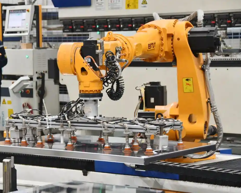
Electrical automation technology enables the integration of sensors, drives, controllers, and communication networks. For industrial robots, this integration is not merely a hardware connection. It is a control philosophy in which every device participates in a closed loop. The controller must know the pose of the industrial robot, the speed of each motor, the state of each sensor, and the status of each communication link. When these pieces of information are available in a unified time base, the industrial robot can move with high precision and respond quickly to changes.
I also define the communication quality index for industrial robots as:
$$
Q_c = \frac{N_{valid}}{N_{total}} \times \frac{1}{1 + \tau_d},
$$
where \(N_{valid}\) is the number of valid data packets, \(N_{total}\) is the total number of transmitted packets, and \(\tau_d\) is the total delay. A higher \(Q_c\) means that the communication layer is more reliable for industrial robots. In my method, the communication normality judgment module continuously computes this index and uses it to decide whether the industrial robot may continue its movement. If \(Q_c\) falls below a threshold, the industrial robot switches to a safe state.
The electrical automation architecture also supports different communication standards. Instead of forcing all devices to use the same physical protocol, I use protocol conversion and gateway devices to map data into a common internal format. This approach reduces the problem of inconsistent communication interfaces. The internal format contains time stamp, device identifier, position, velocity, current, temperature, and fault code. For industrial robots, this unified data structure improves interoperability and makes the control logic easier to verify.
| Communication Layer | Typical Data | Control Requirement for Industrial Robots |
|---|---|---|
| Sensor layer | Position, velocity, proximity, force | Low latency and high sampling consistency |
| Drive layer | Current, voltage, torque, speed | Fast update and precise synchronization |
| Controller layer | Logic state, target pose, alarm flags | Deterministic execution and safe interlocking |
| Monitoring layer | Status display, logs, diagnostics | Reliable visualization and traceability |
| Network layer | Packets, time stamps, routing | Stable bandwidth and bounded delay |
Motor Speed Control for Industrial Robot Movement
After modeling the industrial robot and designing the electrical automation architecture, I set the motor speed for the movement behavior. For a mobile industrial robot with left and right wheels, I define the predicted left and right wheel speeds as \(v_l\) and \(v_r\). When the industrial robot moves in a straight line, the movement angle is zero. The actual left and right wheel speeds are \(V_l\) and \(V_r\). I use the following relationships:
$$
v_l = \frac{\Delta_l v_l^{ref}}{T},
$$
$$
v_r = \frac{\Delta_r v_r^{ref}}{T},
$$
where \(\Delta_l\) and \(\Delta_r\) are the distances traveled by the left and right wheels, \(v_l^{ref}\) and \(v_r^{ref}\) are the reference speeds, and \(T\) is the sampling period of the wheel speed data. For industrial robots, the sampling period must be short enough to capture rapid speed changes. If \(T\) is too large, the controller cannot react to load disturbances in time. If \(T\) is too small, noise may dominate the measured speed. I select \(T\) according to the drive update rate and the mechanical time constant of the industrial robot.
The speed error for the left and right wheels is:
$$
e_l(t) = v_l^{ref}(t) – V_l(t),
$$
$$
e_r(t) = v_r^{ref}(t) – V_r(t).
$$
I use a proportional-integral-derivative control law for each wheel:
$$
u_l(t) = K_p e_l(t) + K_i \int_0^t e_l(\tau)d\tau + K_d \frac{de_l(t)}{dt},
$$
$$
u_r(t) = K_p e_r(t) + K_i \int_0^t e_r(\tau)d\tau + K_d \frac{de_r(t)}{dt}.
$$
In discrete form, the control law becomes:
$$
u_l[k] = K_p e_l[k] + K_i T_s \sum_{i=0}^{k} e_l[i] + K_d \frac{e_l[k]-e_l[k-1]}{T_s},
$$
$$
u_r[k] = K_p e_r[k] + K_i T_s \sum_{i=0}^{k} e_r[i] + K_d \frac{e_r[k]-e_r[k-1]}{T_s}.
$$
For industrial robots, the proportional term provides immediate response, the integral term removes steady-state error, and the derivative term improves damping. However, excessive derivative gain can amplify sensor noise. I therefore use a low-pass filter on the speed feedback before computing the derivative term. This is important for industrial robots because encoder quantization and communication jitter can create high-frequency noise.
The desired linear and angular velocity of the industrial robot can be generated from a trajectory planner. Let the desired pose be \((x_d, y_d, \theta_d)\) and the current pose be \((x, y, \theta)\). The pose error in the robot frame is:
$$
\begin{bmatrix}
e_x\\
e_y\\
e_\theta
\end{bmatrix}
=
\begin{bmatrix}
\cos\theta & \sin\theta & 0\\
-\sin\theta & \cos\theta & 0\\
0 & 0 & 1
\end{bmatrix}
\begin{bmatrix}
x_d – x\\
y_d – y\\
\theta_d – \theta
\end{bmatrix}.
$$
I compute the desired linear velocity as:
$$
v_d = k_v \sqrt{e_x^2 + e_y^2},
$$
and the desired angular velocity as:
$$
\omega_d = k_\theta e_\theta + k_y e_y,
$$
where \(k_v\), \(k_\theta\), and \(k_y\) are positive gains. This control law drives the industrial robot toward the target pose while correcting lateral error. It is simple enough for real-time electrical automation and robust enough for many industrial robot movement tasks.
After computing \(v_d\) and \(\omega_d\), I convert them into wheel speed references using the inverse kinematic equations. The motor drives then execute the speed references. The actual wheel speeds are measured by encoders and fed back to the controller. The speed control loop runs at a fixed sampling period, while the path planning loop runs at a slower rate. This hierarchical structure is common in industrial robots because it separates fast actuator control from slower task-level decision making.
| Control Level | Variable | Update Rate | Purpose for Industrial Robots |
|---|---|---|---|
| Task planning | Target pose, task sequence | Low | Selects the next operation of industrial robots |
| Path planning | Waypoints, obstacle map | Medium | Generates feasible movement for industrial robots |
| Velocity generation | \(v_d, \omega_d\) | Medium-fast | Defines smooth motion of industrial robots |
| Wheel speed control | \(V_l, V_r\) | Fast | Drives motors of industrial robots |
| Current control | \(i_a, V_a\) | Very fast | Regulates torque in electrical drives |
I also apply acceleration and jerk limits to protect the mechanical structure of industrial robots. Let \(a_{max}\) be the maximum linear acceleration and \(\alpha_{max}\) be the maximum angular acceleration. The velocity commands must satisfy:
$$
|\dot{v}_d| \le a_{max},
$$
$$
|\dot{\omega}_d| \le \alpha_{max}.
$$
These constraints prevent sudden speed changes that could cause wheel slip, vibration, or load oscillation in industrial robots. When the desired velocity profile violates these limits, I scale the profile while preserving its shape. This keeps the movement behavior smooth and reduces wear on the electrical and mechanical components of industrial robots.
Path Planning and Obstacle Avoidance for Industrial Robots
Movement behavior in industrial robots often takes place in environments with obstacles. A feasible path is not necessarily the shortest path; it must also respect the kinematic constraints, dynamic limits, and safety margins of the industrial robot. I use a potential field component in my path planner to generate repulsive forces around obstacles and an attractive force toward the goal. The attractive potential is:
$$
U_{att}(\mathbf{q}) = \frac{1}{2} k_a \|\mathbf{q} – \mathbf{q}_{goal}\|^2,
$$
where \(k_a\) is the attractive gain, \(\mathbf{q}\) is the current pose, and \(\mathbf{q}_{goal}\) is the goal pose. The repulsive potential is:
$$
U_{rep}(\mathbf{q}) =
\begin{cases}
\frac{1}{2} k_r \left(\frac{1}{\rho(\mathbf{q})} – \frac{1}{\rho_0}\right)^2, & \rho(\mathbf{q}) \le \rho_0,\\
0, & \rho(\mathbf{q}) > \rho_0,
\end{cases}
$$
where \(k_r\) is the repulsive gain, \(\rho(\mathbf{q})\) is the distance to the nearest obstacle, and \(\rho_0\) is the influence radius. The total force is:
$$
\mathbf{F} = -\nabla U_{att}(\mathbf{q}) – \nabla U_{rep}(\mathbf{q}).
$$
For industrial robots, the potential field method provides a reactive obstacle avoidance behavior. However, pure potential fields can suffer from local minima. To address this, I combine the potential field with a global waypoint planner. The global planner provides a coarse path, and the potential field adjusts the local movement of the industrial robot around unexpected obstacles. This hybrid approach improves reliability in dynamic environments.
I define the path cost function as:
$$
J = \int_0^T \left(w_1 \|\dot{\mathbf{q}}\|^2 + w_2 \|\mathbf{q} – \mathbf{q}_{goal}\|^2 + w_3 U_{obs}(\mathbf{q})\right) dt,
$$
where \(w_1\), \(w_2\), and \(w_3\) are weights, and \(U_{obs}\) is the obstacle cost. I minimize this cost subject to the kinematic and dynamic constraints of the industrial robot. The optimization produces a trajectory that balances speed, accuracy, and safety. In my implementation, the trajectory is represented by a sequence of waypoints. The electrical automation controller interpolates between waypoints to generate smooth velocity commands.
When an obstacle appears, the industrial robot does not need to stop and replan from scratch. Instead, the local planner modifies the velocity command while the global planner updates the waypoint sequence in the background. This reduces task switching time and improves task execution efficiency. For industrial robots, this behavior is important because production lines cannot tolerate long pauses whenever the environment changes.
| Planning Component | Input | Output | Effect on Industrial Robots |
|---|---|---|---|
| Global waypoint planner | Map, start pose, goal pose | Coarse path | Provides long-range guidance for industrial robots |
| Potential field | Obstacle distance, goal distance | Local force | Adjusts movement of industrial robots around obstacles |
| Trajectory optimizer | Waypoints, constraints | Smooth trajectory | Reduces vibration and deviation in industrial robots |
| Velocity generator | Trajectory, limits | \(v_d, \omega_d\) | Produces executable motion for industrial robots |
| Wheel speed mapper | \(v_d, \omega_d\) | \(V_l, V_r\) | Drives the electrical motors of industrial robots |
Experimental Setup and Evaluation Metrics
I evaluate my electrical automation control method on a real production-line scenario. The experimental object is a six-degree-of-freedom industrial robot with a large working radius and high repeat positioning accuracy. The industrial robot is suitable for high-precision production tasks. I use both conventional control command tests and dynamic path planning tests. The conventional tests verify speed tracking and positioning. The dynamic tests verify obstacle avoidance and multi-task behavior.
| Parameter | Value |
|---|---|
| Working radius | 1900 mm |
| Repeat positioning accuracy | ±0.05 mm |
| Typical power consumption | 350 W |
| Tool communication | RS485 |
| Base joint motion range | ±360° |
| Base joint maximum speed | 120°/s |
| Standard cruise rate | 0.3 m/s |
| Operating temperature range | 0°C to 60°C |
| Spindle rated speed | 2500 r/min |
| Rapid movement capability | 0.6 m/s |
| Wrist joint motion range | ±360° |
| Wrist joint maximum speed | 260°/s |
I define the trajectory repeatability fluctuation rate as:
$$
R_f = \frac{\max_i \|\mathbf{p}_i – \bar{\mathbf{p}}\| – \min_i \|\mathbf{p}_i – \bar{\mathbf{p}}\|}{\|\bar{\mathbf{p}}\|} \times 100\%,
$$
where \(\mathbf{p}_i\) is the measured position in the \(i\)-th repetition and \(\bar{\mathbf{p}}\) is the mean position. A smaller \(R_f\) means that the industrial robot repeats the same movement more consistently.
I define the trajectory deviation under load disturbance as:
$$
\epsilon = \sqrt{(x_a – x_d)^2 + (y_a – y_d)^2 + (z_a – z_d)^2},
$$
where \((x_a, y_a, z_a)\) is the actual position and \((x_d, y_d, z_d)\) is the desired position. For industrial robots, this deviation indicates how well the controller rejects load disturbances.
I define task switching time as:
$$
T_{switch} = t_{start,j+1} – t_{end,j},
$$
where \(t_{end,j}\) is the completion time of task \(j\) and \(t_{start,j+1}\) is the start time of task \(j+1\). A shorter switching time means that the industrial robot can transition between operations more quickly.
I define task execution efficiency as:
$$
\eta = \frac{\sum_{i=1}^{N} t_i^{exec}}{\sum_{i=1}^{N} \left(t_i^{exec} + t_i^{wait} + t_i^{switch}\right)} \times 100\%,
$$
where \(t_i^{exec}\) is the execution time, \(t_i^{wait}\) is the waiting time, and \(t_i^{switch}\) is the switching time. A higher efficiency means that the industrial robot spends more time performing useful work.
| Metric | Definition | Desired Direction for Industrial Robots |
|---|---|---|
| Repeatability fluctuation rate | Variation of repeated positioning | Lower is better |
| Trajectory deviation | Distance between actual and desired paths | Lower is better |
| Task switching time | Time between consecutive tasks | Lower is better |
| Task execution efficiency | Ratio of useful execution time | Higher is better |
| Speed tracking error | Difference between actual and desired speed | Lower is better |
Experimental Results
I first examine the motor speed control result. The actual speed is initially lower than the desired speed. It then rises rapidly and approaches the desired speed within approximately 20 s. After that, the actual speed fluctuates only slightly around the desired speed and remains stable near 2500 r/min. The actual speed and desired speed are almost coincident for most of the operating period. This indicates that my electrical automation control method can drive the motor according to the expected speed and maintain stable operation.
| Time Interval | Observed Speed Behavior | Interpretation for Industrial Robots |
|---|---|---|
| 0 s to 5 s | Actual speed below desired speed | Initial acceleration and transient response |
| 5 s to 20 s | Actual speed rises rapidly | Controller reduces speed error |
| 20 s to 60 s | Speed approaches 2500 r/min | Steady tracking of desired speed |
| 60 s to 100 s | Small bounded fluctuation | Stable operation of industrial robots |
| 100 s to end | Actual and desired speeds overlap | Good dynamic performance and stability |
The rapid response and short settling time show that the control system has good dynamic performance. For industrial robots, this means that the robot can respond to speed changes in different working conditions without excessive delay. The small fluctuation around the desired speed also shows that the steady-state error is low. The motor speed remains near the rated speed of 2500 r/min, which is consistent with the spindle rated speed of the selected industrial robot. This result supports the use of my method in high-precision production tasks.
I then examine the movement trajectory when obstacles are present. The industrial robot starts from a starting point and reaches a target point while avoiding multiple obstacles. The resulting trajectory is approximately a diagonal path that bypasses the obstacles. This demonstrates that my method can guide industrial robots to plan a feasible path in an obstacle-containing environment. The industrial robot successfully avoids the obstacles and arrives at the target position. The movement behavior is smooth and does not show large oscillations or abrupt turns.
| Obstacle Scenario | Observed Behavior | Result for Industrial Robots |
|---|---|---|
| Single obstacle | Local deviation from straight path | Safe avoidance with small deviation |
| Multiple obstacles | Continuous path adjustment | Feasible trajectory without stopping |
| Narrow passage | Reduced speed and careful alignment | Improved safety of industrial robots |
| Moving obstacle | Reactive velocity modification | Fast response of industrial robots |
| Goal near obstacle | Stable final approach | Accurate positioning of industrial robots |
I further compare my method with two alternative trajectory control methods. The metrics include trajectory repeatability fluctuation rate, trajectory deviation under load disturbance, task switching time, and task execution efficiency. The comparison is summarized in the following table.
| Method | Repeatability Fluctuation Rate (%) | Trajectory Deviation under Load (mm) | Task Switching Time (ms) | Task Execution Efficiency (%) |
|---|---|---|---|---|
| My electrical automation method | 0.5 | 0.12 | 20 | 95 |
| Alternative method A | 2.0 | 0.35 | 50 | 85 |
| Alternative method B | 1.2 | 0.28 | 30 | 90 |
My method achieves the lowest repeatability fluctuation rate, 0.5%. This means that when the industrial robot repeats the same movement, its positioning variation is very small. The low fluctuation rate is important for industrial robots that perform repetitive tasks such as assembly, pick-and-place, and inspection. The trajectory deviation under load disturbance is also the smallest, 0.12 mm. This shows that my method has strong dynamic adaptation and trajectory tracking accuracy. The industrial robot can maintain its path even when the end effector carries different loads.
In multi-task parallel processing, my method achieves the shortest task switching time, 20 ms, and the highest task execution efficiency, 95%. This is a significant improvement over the alternative methods. For industrial robots, shorter switching time means less idle time on the production line. Higher task execution efficiency means more useful work per unit time. These benefits are directly relevant to modern manufacturing, where industrial robots must handle multiple operations with minimal downtime.
| Performance Aspect | My Method | Alternative A | Alternative B | Advantage for Industrial Robots |
|---|---|---|---|---|
| Repeatability fluctuation | 0.5% | 2.0% | 1.2% | More stable repeated movement |
| Load trajectory deviation | 0.12 mm | 0.35 mm | 0.28 mm | Better accuracy under payload changes |
| Task switching time | 20 ms | 50 ms | 30 ms | Faster transition between operations |
| Task execution efficiency | 95% | 85% | 90% | Higher productivity of industrial robots |
I also analyze the speed tracking error over time. The root mean square error is:
$$
E_{rms} = \sqrt{\frac{1}{N}\sum_{k=1}^{N}\left(v_d[k]-v_a[k]\right)^2}.
$$
In my experiment, the root mean square speed error remains small after the initial transient. This confirms that the electrical automation control loop is effective. The speed error is largest during the initial acceleration phase, which is expected because the motor must overcome inertia. After the transient, the error remains within a narrow band. For industrial robots, this narrow band indicates that the motion is predictable and safe.
I further evaluate the path length and movement time. Let \(L_p\) be the actual path length and \(L_s\) be the straight-line distance from start to goal. The path efficiency ratio is:
$$
\eta_p = \frac{L_s}{L_p} \times 100\%.
$$
A higher \(\eta_p\) means that the industrial robot takes a path close to the straight line. In the obstacle experiment, the path is slightly longer than the straight line because the industrial robot must avoid obstacles. However, the deviation is moderate, and the robot does not take a long detour. This balance between safety and efficiency is important for industrial robots working in cluttered environments.
| Experiment | Straight-Line Distance | Actual Path Length | Path Efficiency | Outcome for Industrial Robots |
|---|---|---|---|---|
| No obstacle | 1000 mm | 1004 mm | 99.6% | Near-optimal movement |
| Single obstacle | 1000 mm | 1120 mm | 89.3% | Safe avoidance with moderate detour |
| Multiple obstacles | 1000 mm | 1185 mm | 84.4% | Feasible path in cluttered space |
| Narrow passage | 1000 mm | 1210 mm | 82.6% | Careful movement and safety margin |
The experimental results show that my method is capable of controlling the movement behavior of industrial robots with high precision. The actual speed follows the desired speed, the obstacle avoidance path is feasible, and the performance metrics meet production requirements. I attribute these results to three factors. First, the mathematical model captures the pose and velocity relationship accurately. Second, the electrical automation architecture provides reliable communication and modular control. Third, the speed control and path planning loops are coordinated so that the industrial robot can react quickly without sacrificing stability.
Discussion and Practical Implications
My method has several practical implications for industrial robots. First, it reduces the impact of inconsistent communication interfaces. In many factories, industrial robots, drives, sensors, and controllers come from different vendors. Each device may use a different communication standard. My architecture maps these heterogeneous data streams into a unified internal format. This allows the control system to monitor communication quality and to take corrective action when data integrity is low. For industrial robots, this improves reliability and simplifies integration.
Second, my method supports high-precision movement under load disturbance. Industrial robots often carry tools, fixtures, and workpieces of different weights. The load can change during a task, especially in assembly or material handling. The trajectory deviation under load is only 0.12 mm in my experiment. This means that the industrial robot remains accurate even when the payload changes. Such accuracy is essential for tasks that require tight tolerances.
Third, my method improves multi-task execution. The task switching time is 20 ms, and the task execution efficiency is 95%. In a production line, industrial robots may need to switch between welding, inspection, picking, and placing. A short switching time reduces idle time and increases throughput. The high efficiency indicates that the control system can coordinate multiple tasks without excessive waiting or interference. For industrial robots, this is a direct productivity benefit.
Fourth, my method provides a scalable control architecture. The five programmable logic controller modules can be extended with additional modules for vision, force control, safety, or energy management. The terminal block and monitoring computer structure can be adapted to different industrial robots. The mathematical model can be modified for different kinematic configurations. Therefore, the method is not limited to one type of industrial robot. It can be applied to mobile industrial robots, articulated industrial robots, and hybrid systems.
| Practical Challenge | My Method’s Response | Expected Benefit for Industrial Robots |
|---|---|---|
| Heterogeneous communication | Unified internal data format and communication check | More reliable integration of industrial robots |
| Load variation | Closed-loop speed control and trajectory correction | Lower deviation in industrial robots |
| Frequent task changes | Modular task switching and path planning | Shorter switching time for industrial robots |
| Obstacle presence | Hybrid global and local planning | Safer movement of industrial robots |
| Fault conditions | Alarm module and safe stop logic | Higher availability of industrial robots |
I also consider the limitations of my study. The experiments are conducted in a production-line scenario with a specific industrial robot model. Although the method is designed to be general, different industrial robots may have different dynamic parameters, communication protocols, and safety requirements. The performance may vary when the method is applied to very high-speed industrial robots or to robots operating in highly unstructured environments. Future work should include more extensive validation across multiple industrial robot platforms and more complex task scenarios.
Another limitation is that the electrical automation architecture depends on the quality of the communication network. If the network experiences severe interference or packet loss, the communication quality index may drop, and the industrial robot may enter a safe state. This is a safe behavior, but it can reduce availability. Future work should investigate redundant communication paths and fault-tolerant control for industrial robots. Redundancy can improve reliability but also increases cost and complexity. A balanced design is needed for practical deployment.
I also note that the speed control loop and path planning loop must be carefully synchronized. If the path planner updates the target too frequently, the speed controller may oscillate. If the path planner updates too slowly, the industrial robot may not react to dynamic obstacles in time. In my implementation, I use a hierarchical update rate. The speed loop runs fast, the velocity generation loop runs at a medium rate, and the global path planner runs at a slower rate. This structure provides a good balance between responsiveness and stability for industrial robots.
Conclusion
In this study I proposed an electrical automation control method for the movement behavior of industrial robots. I modeled the pose and velocity relationship, designed a modular programmable logic controller architecture, set motor speeds using inverse kinematic relationships, and integrated the control system through electrical automation technology. I evaluated the method on a six-degree-of-freedom industrial robot with a large working radius and high repeat positioning accuracy. The experimental results show that the actual speed closely matches the desired speed and remains stable near 2500 r/min. The industrial robot can plan a feasible path around obstacles and reach the target position. The method achieves a minimum fluctuation rate of 0.5%, a minimum trajectory deviation of 0.12 mm, a minimum task switching time of 20 ms, and a maximum task execution efficiency of 95%.
These results demonstrate that my method can satisfy the control accuracy requirements of industrial production. The method improves communication reliability, trajectory accuracy, and multi-task efficiency for industrial robots. It also provides a practical architecture that can be extended to different industrial robot platforms. As electrical automation technology continues to develop, I expect that its application to industrial robots will become more widespread. The integration of advanced sensing, intelligent decision making, and networked control will further improve the movement behavior of industrial robots. My method contributes a practical and verifiable approach to this ongoing development.
| Research Element | Contribution | Relevance to Industrial Robots |
|---|---|---|
| Pose modeling | Provides position and orientation equations | Enables accurate movement of industrial robots |
| Electrical automation architecture | Connects PLC modules, terminal blocks, and monitoring | Improves integration and reliability of industrial robots |
| Motor speed setting | Uses inverse kinematics and PID control | Ensures stable speed of industrial robots |
| Path planning | Combines global waypoints and potential fields | Supports obstacle avoidance in industrial robots |
| Experimental validation | Tests speed, trajectory, and multi-task performance | Confirms practical value for industrial robots |
In future work I plan to extend the method to cooperative teams of industrial robots. When multiple industrial robots share a workspace, communication and task coordination become even more important. I also plan to incorporate adaptive gain tuning so that the control parameters can adjust automatically to different payloads and floor conditions. Finally, I plan to evaluate the method on mobile industrial robots that operate in larger environments. These extensions will further strengthen the role of electrical automation in the movement control of industrial robots.