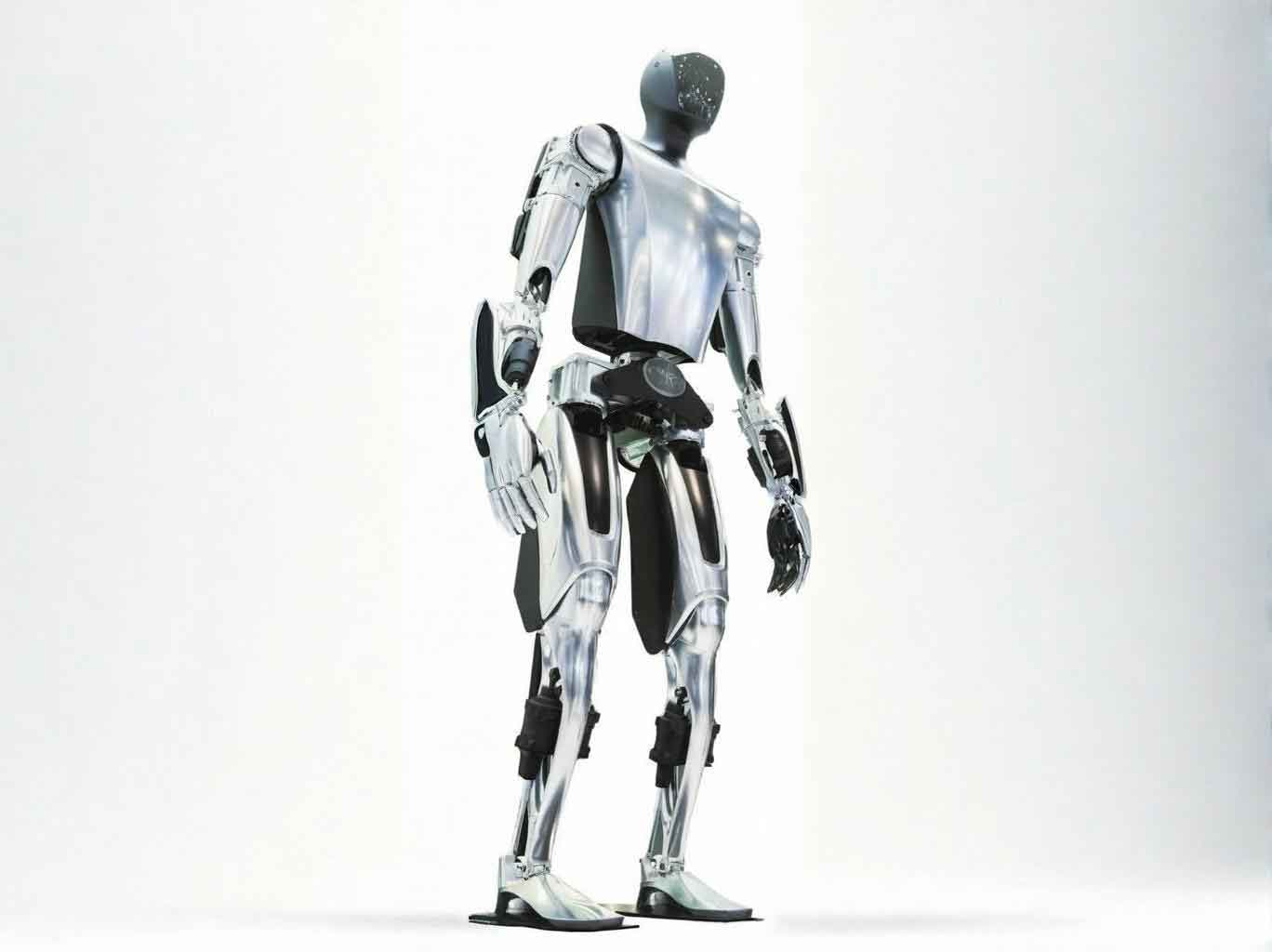
This dissertation presents a comprehensive study on gait planning and anti-push control for a biped humanoid robot as an embodiment of an embodied robot. The work integrates the linear inverted pendulum model (LIPM), kinematic modeling, and capture-point theory to achieve stable locomotion and disturbance recovery. A 20-degree-of-freedom (DOF) biped humanoid robot is modeled, simulated, and experimentally validated on a physical platform. The gait planning method is based on the LIPM in both the coronal and sagittal planes, with an improved foot trajectory that reduces landing impact. The anti-push algorithm employs the concept of orbital energy and capture points, enabling the robot to recover from external pushes during standing and stepping tasks. Simulation results demonstrate the effectiveness of the proposed methods, and the physical experiments confirm the robustness of the gait planner across various ground surfaces. The study highlights the importance of embodied robot design and control for real-world applications.
1. Introduction
The development of embodied robot systems has gained significant attention due to their potential to operate in human-centered environments. Among various embodiments, biped humanoid robots closely mimic human morphology and locomotion, offering superior adaptability to stairs, doors, and other human-oriented structures. However, achieving stable bipedal walking and maintaining balance under external disturbances remain challenging tasks. Traditional gait planning methods, such as zero-moment point (ZMP) based approaches, linear inverted pendulum model (LIPM), and central pattern generators (CPG), have been widely studied. Nevertheless, many bipedal robots still lack the ability to respond to external pushes or uneven terrains, especially small-scale embedded systems.
The primary objective of this research is to develop a robust gait planning algorithm and an anti-push recovery strategy for a small-scale biped humanoid robot. The proposed approach leverages the LIPM for its computational efficiency and the capture-point theory for its practical applicability in real-time control. The work is structured as follows:
- Construction of a 20-DOF biped humanoid robot model and kinematic analysis using forward and inverse kinematics.
- Application of the LIPM to generate center-of-mass (CoM) trajectories in the coronal and sagittal planes, along with foot trajectory planning for swing and support phases.
- Improvement of the swing foot trajectory to minimize landing impact and enhance walking stability.
- Implementation of the gait planner in a V-REP/ROS simulation environment and validation on a physical robot platform across different ground surfaces.
- Development of an anti-push controller based on orbital energy and capture-point theory, followed by simulation verification.
This research contributes to the field of embodied robot control by providing a systematic framework for bipedal locomotion that is both computationally lightweight and experimentally feasible for small-scale robots.
2. Kinematics and Inverted Pendulum Model
The embodied robot under study is modeled with 20 degrees of freedom, as shown in the schematic representation. Each leg has six DOFs, while the torso, arms, and head contribute additional DOFs. For gait control, the leg joints are of primary interest, and the upper body DOFs are kept at constant angles during walking.
| Body Part | Number of DOFs |
|---|---|
| Each leg | 6 |
| Torso | 2 |
| Each arm | 3 |
| Head | 2 |
| Total | 20 |
2.1 Inverse Kinematics
The inverse kinematics (IK) problem is solved analytically for one leg chain. Given the desired pose of the torso relative to the ankle, the joint angles are computed. For the right leg, the hip position in the ankle coordinate frame is expressed as:
$$ \mathbf{r} = [r_x, r_y, r_z]^T = {}^7 R \left( \mathbf{p} – {}^2 \mathbf{p} \right) $$
where \( \mathbf{p} \) is the torso position, \( {}^2 \mathbf{p} \) is the hip position, and \( {}^7 R \) is the rotation matrix from the ankle to the hip. The distance \( C \) between hip and ankle is given by:
$$ C = \sqrt{r_x^2 + r_y^2 + r_z^2} $$
Applying the law of cosines to the leg linkage with thigh length \( A \) and shank length \( B \), the knee angle \( q_5 \) is obtained:
$$ q_5 = \pi – \arccos\left( \frac{A^2 + B^2 – C^2}{2AB} \right) $$
The ankle pitch and roll angles \( q_6 \) and \( q_7 \) are then derived using:
$$ q_7 = \arctan(r_y, r_z) $$
$$ q_6 = \arctan\left( r_x, \sqrt{r_y^2 + r_z^2} \right) – \alpha $$
with \( \alpha \) determined from the sine law. Finally, the hip joint angles \( q_1 \) to \( q_4 \) are solved from the rotation matrix equation:
$$ {}^7 R = R_z(q_1) R_y(q_2) R_x(q_3) R_y(q_4) R_x(q_5) R_y(q_6) R_z(q_7) $$
The resulting angles are expressed as:
$$ q_1 = \arctan(-R_{12}, R_{22}) $$
$$ q_2 = \arctan( R_{32}, R_{12} \sin q_1 + R_{22} \cos q_1 ) $$
$$ q_3 = \arctan( -R_{31}, R_{33} ) $$
The same procedure is applied to the left leg with a mirrored configuration.
2.2 Linear Inverted Pendulum Model
The linear inverted pendulum model abstracts the robot’s dynamics into a point mass concentrated at the CoM, supported by a massless telescopic leg. The equation of motion projected on a horizontal plane is:
$$ \ddot{x} = \frac{g}{H} x = \omega^2 x $$
where \( H \) is the constant CoM height, \( g \) is gravitational acceleration, and \( \omega = \sqrt{g/H} \). The general solution for position and velocity is:
$$ x(t) = x_0 \cosh(\omega t) + \frac{v_0}{\omega} \sinh(\omega t) $$
$$ v(t) = x_0 \omega \sinh(\omega t) + v_0 \cosh(\omega t) $$
These equations form the basis for generating the CoM trajectories in the coronal and sagittal planes.
3. Gait Planning Based on the Inverted Pendulum Model
3.1 CoM Trajectory in the Coronal Plane
During the support phase, the CoM behaves like an inverted pendulum pivoting about the supporting ankle. For a half-step period \( T/2 \), with a constant distance \( D \) between the two feet, the CoM starts and ends at \( \pm D/2 \) with zero velocity. The initial velocity \( v_0 \) is determined by imposing these boundary conditions:
$$ v_0 = \frac{D \omega (1 – \cosh(\omega T/2))}{2 \sinh(\omega T/2)} $$
The resulting CoM trajectory in the coronal plane is a hyperbolic cosine-like curve, as illustrated conceptually in the simulation results.
3.2 CoM Trajectory in the Sagittal Plane
For a forward step length \( F \), the CoM moves from \( -F/4 \) to \( F/4 \) during one support phase. The initial velocity is:
$$ v_0 = \frac{F \omega (1 + \cosh(\omega T/2))}{4 \sinh(\omega T/2)} $$
The CoM position in the sagittal plane follows the same hyperbolic form, providing a natural forward acceleration and deceleration pattern.
3.3 Swing Foot Trajectory
In the coronal plane, the swing foot maintains a constant lateral position relative to the torso. In the sagittal plane, the foot moves from \( -F/4 \) to \( F/4 \) during half a walking cycle. A sinusoidal profile is selected to ensure smooth motion:
$$ y(t) = \frac{F}{4} \sin\left( \frac{2\pi t}{T} \right) $$
For the vertical direction, an initial trajectory was set as:
$$ z(t) = H_0 \sin\left( \frac{2\pi t}{T} \right) $$
where \( H_0 \) is the maximum foot clearance. This simple sinusoidal profile caused significant CoM oscillation upon landing. To reduce impact, the vertical trajectory was redesigned as a piecewise function:
$$ z(t) = \begin{cases}
\frac{H_0}{2} \sin\left( \frac{4\pi t}{T} \right), & 0 \le t < \frac{T}{4} \\
\frac{H_0}{2} + \frac{H_0}{2} \sin\left( \frac{4\pi (t – T/4)}{T} \right), & \frac{T}{4} \le t \le \frac{T}{2}
\end{cases} $$
This modified trajectory gives a steeper takeoff and a gentler touchdown, thereby minimizing the impact force at landing. Simulation results confirmed that the vertical CoM oscillation is considerably reduced.
3.4 Simulation Setup
The control system for the embodied robot is illustrated as a feedback loop. A gait planner generates CoM and foot trajectories, which are fed to an IK-based angle resolver. The resolver computes the twelve leg joint angles (six for each leg) and sends them to the V-REP simulator. The simulator uses the TALOS robot model with the following properties:
| Parameter | Value |
|---|---|
| Total height | 0.65 m |
| Total mass | 5.386 kg |
| Thigh length | 0.136 m |
| Shank length | 0.136 m |
| Foot length × width | 0.16 m × 0.14 m |
| CoM height | 0.36 m |
The walking cycle was set to \( T = 1.6 \, \text{s} \), and the control loop ran at 50 Hz. Joint angles generated by the IK solver were applied to the virtual robot, resulting in stable walking. Figure 1 shows the simulated walking sequence. The improved foot trajectory produced a smoother vertical CoM profile compared to the original sinusoidal trajectory, as depicted in the local amplification comparison.
The simulated embodied robot successfully walked forward with a step length of 0.1 m and a step height of 0.04 m. The CoM remained close to the constant height, confirming the effectiveness of the modified swing trajectory.
3.5 Experimental Implementation
After verifying the gait in simulation, physical experiments were conducted on the TALOS robot platform, which matched the simulation model in all geometric and mass properties. The robot was placed on different ground surfaces: a hard desktop, a hard carpet, and a rubber pad. The joint angles obtained from the planner were sent to the servo motors, and the robot performed stepping motions. During the initial tests, the robot exhibited slight instability due to inadequate servo torque. To counteract this, a numerical compensation was applied to the commanded joint angles, effectively adjusting for servo backlash and deflection. The compensation values were determined empirically and fine-tuned to ensure stable motion.
Figure 2 shows the physical robot walking on different surfaces. The lateral CoM trajectory measured from the encoders closely matched the theoretical curve, with minor deviations during the first step. The robot maintained balance and completed multiple steps without falling, demonstrating the robustness of the gait planner.
3.6 Disturbance Rejection of the Gait Planner
The inherent robustness of the LIPM-based gait was tested by applying lateral and forward pushes during walking in simulation. A force of 3 N in the lateral direction and 4 N in the backward direction was applied at \( t = 2.2 \, \text{s} \). The resulting CoM trajectories are shown in Figure 3. After the push, the CoM deviated from the nominal path but recovered within two walking cycles. However, when the push magnitude was increased to 10 N, the robot fell during the single-support phase, confirming that the base gait lacks active push recovery.
4. Anti-Push Control Based on Capture Point
4.1 Push Disturbance Characterization
An external push is characterized by its direction, onset time, duration, and momentum. In this study, we consider a short-duration push (less than one-fifth of the walking cycle) that imparts a sudden momentum change to the CoM. The push is assumed to act horizontally through the CoM.
| Attribute | Description |
|---|---|
| Direction | Any horizontal direction |
| Onset time | Any time during the gait cycle |
| Duration | Short (impulsive) |
| Momentum magnitude | Determines the disturbance severity |
4.2 Orbital Energy
The orbital energy of the linear inverted pendulum is defined as:
$$ E = \frac{1}{2}m\dot{x}^2 – \frac{1}{2}m\omega^2 x^2 $$
This energy is constant during undisturbed motion. When a push occurs, the orbital energy changes instantaneously. By measuring the CoM position and velocity, the current orbital energy can be computed. A disturbance is detected when the energy deviation exceeds a preset threshold:
$$ |E(t) – E_0| > \Delta E $$
where \( E_0 \) is the nominal orbital energy of the desired gait and \( \Delta E \) is the threshold.
4.3 Capture Point for Static State
For a static robot that receives a push, the capture point is defined as the foot placement location that brings the orbital energy back to zero. From the energy equation, setting \( E=0 \) yields:
$$ \frac{1}{2} m v_p^2 – \frac{1}{2} m \omega^2 x_{cp}^2 = 0 \Rightarrow x_{cp} = \frac{v_p}{\omega} $$
In practice, the robot needs a finite stepping time \( t_p \). During that time, the CoM moves due to gravity. Accounting for this, the capture point is:
$$ x_{cp} = x_p \cosh(\omega t_p) + \frac{v_p}{\omega} \sinh(\omega t_p) + \frac{v_p \cosh(\omega t_p) + \omega x_p \sinh(\omega t_p)}{\omega} $$
where \( x_p \) and \( v_p \) are the CoM position and velocity at the moment the push is detected. This formula provides the exact foot location that achieves a balanced state after stepping.
4.4 Capture Point for Moving State
For a moving robot, the orbital energy is not generally zero. The goal is to recover the nominal orbital energy \( E_0 \) associated with the desired motion. Consider a robot walking in the forward direction. The total motion can be decomposed into an acceleration phase (when the CoM moves away from the support foot) and a deceleration phase (when it moves toward the next support foot). Let \( x_{acc} \) be the distance traveled in the acceleration phase and \( x_{dec} \) in the deceleration phase. The orbital energy after the push and after stepping are related by:
$$ E_2 = E_1 + \frac{1}{2} m\omega^2 (x_{acc}^2 – x_{dec}^2) $$
To recover \( E_0 \), we need \( x_{dec} > x_{acc} \) if \( E_1 > E_0 \). The controller adjusts the step length and stepping time to achieve this. The desired step location \( x_s \) is computed by combining the push-detection state and the desired terminal velocity.
Let the cycle starting point be \( x_n \). The CoM state at the push instant is \( (x_p, v_p) \). The new step is to be placed at \( x_s \). The time to foot placement \( t_p \) is predetermined. After stepping, the CoM position is \( x_d \), and the velocity is \( v_d \). The relation between the states and the foot position is:
$$ x_d = x_p \cosh(\omega t_p) + \frac{v_p}{\omega} \sinh(\omega t_p) $$
$$ v_d = x_p \omega \sinh(\omega t_p) + v_p \cosh(\omega t_p) $$
The desired orbital energy after stepping should equal \( E_0 \), which gives:
$$ E_0 = \frac{1}{2} m v_d^2 – \frac{1}{2} m\omega^2 (x_d – x_s)^2 $$
Solving for \( x_s \):
$$ x_s = x_d + \frac{\sqrt{v_d^2 – 2 E_0/m}}{\omega} $$
This expression is subject to the physical limit of the robot’s leg reach. If \( x_s \) exceeds the maximum step length \( x_{lim} \), the robot takes the maximum possible step and may need multiple steps to fully recover.
4.5 Anti-Push Control Algorithm
The complete anti-push control algorithm is summarized as follows:
- Measure the CoM position \( x(t) \) and velocity \( v(t) \) in real time.
- Compute the current orbital energy \( E(t) \) and compare it with the nominal value \( E_0 \). If the deviation is below the threshold, continue normal gait planning.
- If a push is detected, set the initial state \( (x_p, v_p) \) and the stepping time \( t_p \).
- Compute the desired step location \( x_s \) using the moving-state capture point formula.
- Check whether \( x_s \le x_{lim} \). If yes, execute the step to \( x_s \). If not, set \( x_s = x_{lim} \), perform the step, and repeat the process for the next step.
- After each recovery step, update the orbital energy and confirm that it has returned to \( E_0 \). Terminate the recovery routine when the robot is back to the nominal gait cycle.
The stepping time \( t_p \) is a critical parameter. Too small a \( t_p \) may exceed the servo speed limit, while too large a \( t_p \) may cause the robot to fall before completing the step. In the simulation, \( t_p = 0.6 \, \text{s} \) was selected as a compromise.
5. Simulation Results of Anti-Push Recovery
5.1 Experimental Setup in Simulation
Simulations were carried out using the same 20-DOF virtual prototype. The robot was initially commanded to perform an in-place stepping motion, characterized by alternating support legs without forward translation. A push force vector of \( 30 \, \text{N} \) in the \( x \)-direction and \( 40 \, \text{N} \) in the \( -y \)-direction was applied at \( t = 1.35 \, \text{s} \). This push was equivalent to a combined impulse of magnitude 50 N (if the duration is 1 s, the impulse is 50 N·s). The anti-push controller was enabled, and the desired foot placement was computed in real time.
5.2 Comparison of With and Without Anti-Push Control
The same push was applied in two scenarios: one with the anti-push controller active, and one with the controller disabled. Figure 4 shows the CoM trajectories in the coronal and vertical planes for the uncontrolled case. The robot lost its balance immediately after the push and fell to the ground. The vertical CoM position dropped quickly, confirming a fall scenario.
In contrast, when the anti-push controller was active, the robot executed a quick step to the computed capture point. The CoM trajectories are shown in Figure 5. Although the vertical CoM dipped slightly due to the step motion, it quickly recovered to the nominal height. The lateral (coronal) CoM offset reached a maximum of about 4 cm but then returned to the original oscillation around the center. The sagittal (forward) CoM motion remained stable, and the robot continued stepping in place after the recovery.
The capture point computation for this scenario yielded a foot placement of approximately \( x_{cp} = 8.5 \, \text{cm} \) in the coronal direction and \( y_s = 12.3 \, \text{cm} \) in the sagittal direction. These values were within the physical limits of the robot, enabling a single-step recovery.
5.3 Large Push and Multiple Step Recovery
When the push was increased to \( 30 \, \text{N} \) in \( x \) and \( 150 \, \text{N} \) in \( -y \), the computed capture point exceeded the robot’s maximum step length. The robot attempted to step to the limit \( x_{lim} \), but the remaining energy was too high to dissipate in a single step. Consequently, the robot fell, as shown in Figure 6. This outcome highlights the limitation of the proposed method for very large disturbances.
For intermediate push magnitudes that require more than one step but do not immediately cause a fall, the algorithm can be extended to a multi-step recovery. The simulation of a two-step recovery case is presented in Figure 7, where the robot takes two consecutive steps before returning to its nominal stepping pattern.
6. Physical Experiments on the Embodied Robot
The gait planning algorithm was tested on the physical TALOS robot. Three surface types were used: a hard wooden table, a low-pile carpet, and a rubber exercise mat. The robot executed a stepping-in-place motion and a forward walking motion. The joint angle compensation was applied to counteract torque deficiencies in the servos.
| Surface | Friction Coefficient | Stepping Speed (steps/min) | Stability (subjective) |
|---|---|---|---|
| Hard desktop | 0.2 | 37 | Excellent |
| Hard carpet | 0.4 | 37 | Good |
| Rubber pad | 0.8 | 37 | Excellent |
The experimental results confirmed that the proposed LIPM-based gait planner is robust enough to handle varying friction conditions. The measured CoM trajectory in the coronal plane closely matched the theoretical curve, as shown in Figure 8. The small deviations during the initial transient were attributed to the lack of an active balance controller, yet the robot did not fall.
It is worth noting that the anti-push algorithm was only verified in simulation due to hardware limitations. The physical robot did not have force/torque sensors sufficient for real-time push detection. Therefore, the anti-push results are presented as a simulation study, which still provides valuable insight for future embedded implementations.
7. Discussion
The proposed framework demonstrates that a lightweight LIPM-based approach can achieve stable bipedal locomotion for a small embodied robot. The improved swing foot trajectory significantly reduces landing impact, which is critical for maintaining the CoM height. The anti-push controller based on orbital energy and capture points provides a practical solution for push recovery, as long as the push magnitude does not exceed the physical limits of the robot.
The embodied robot concept emphasizes the integration of physical embodiment, real-time sensing, and adaptive control. In this work, the robot’s embodiment parameters—such as link lengths, masses, and actuator limits—were explicitly considered in the trajectory planning and control. Future work will focus on extending the anti-push algorithm to the physical platform by incorporating torque sensors and faster servo systems.
8. Conclusion
This dissertation presented a systematic approach to gait planning and anti-push control for a biped humanoid robot as an embodied robot. The key contributions are:
- An analytical inverse kinematics solution for a 20-DOF biped robot, enabling efficient joint angle computation from CoM and foot trajectories.
- A linear inverted pendulum-based gait planner that generates stable CoM and foot trajectories in both the coronal and sagittal planes.
- An improved swing foot trajectory that reduces landing impact and improves vertical CoM stability.
- A successful simulation and physical implementation of the gait planner on a small-scale robot, with stable locomotion across multiple ground surfaces.
- An anti-push controller based on orbital energy and capture-point theory, validated in simulation for both static and dynamic recovery scenarios.
The results demonstrate the feasibility of deploying lightweight, computationally efficient algorithms on small-scale embodied robots for advanced locomotion and disturbance rejection. The findings contribute to the broader goal of making bipedal robots more adaptable to real-world environments.