
1. Introduction
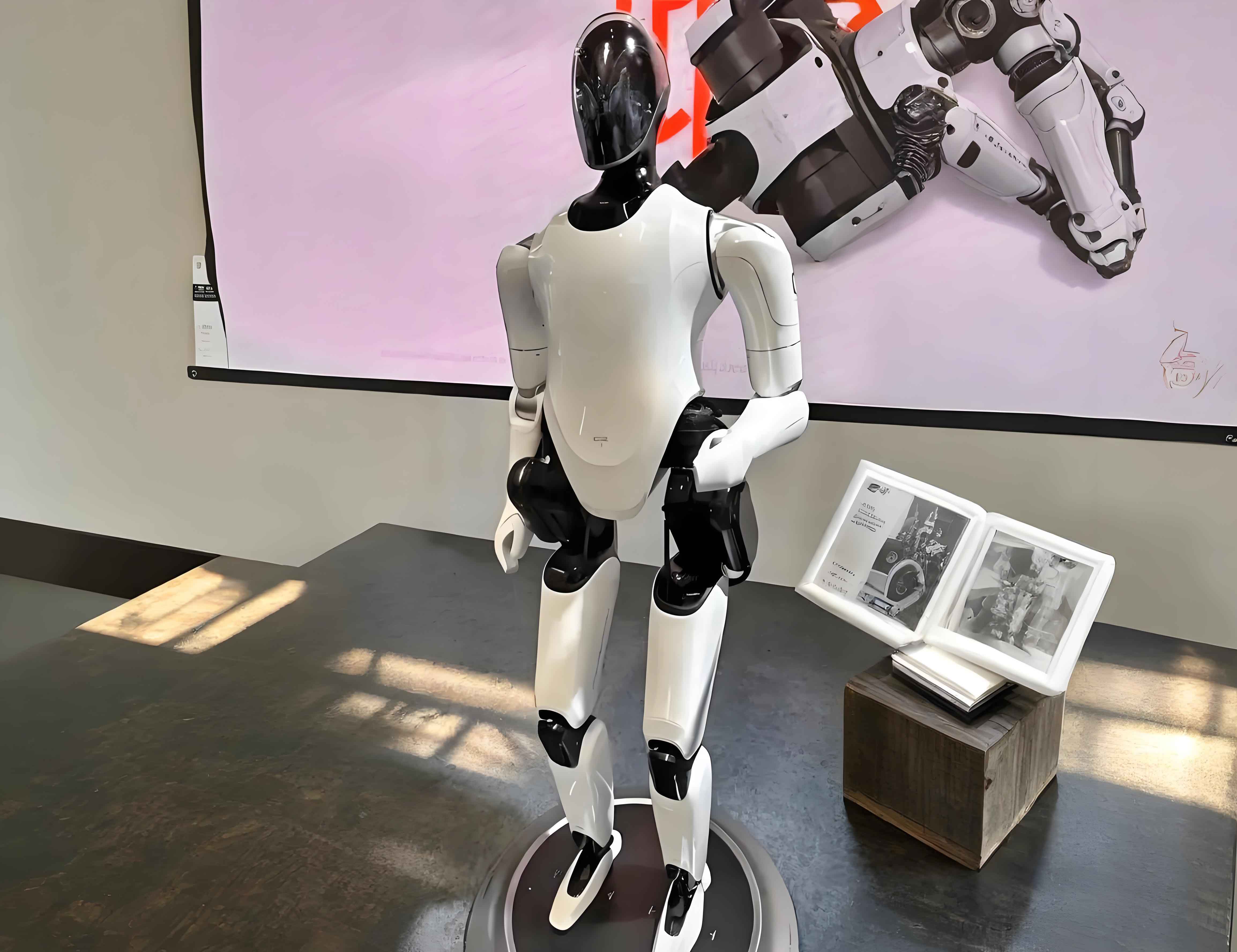
In 2024, the humanoid robot sector experienced explosive growth, transitioning from relative obscurity to a leading technological trend. The field of embodied robot research has gained significant momentum, with applications expanding from industrial environments into human-centric settings. This shift presents substantial challenges in control theory, hardware-software integration, and system design.
The study of humanoid robots began in the last century, yet progress was constrained by limitations in control theory and hardware technology. However, recent years have marked a critical opportunity for the development of embodied robot platforms. The fundamental requirement for humanoid robots is to achieve stable bipedal locomotion similar to humans. This primary requirement encompasses two critical research areas: stability maintenance and gait generation.
While industrial robots operate in structured environments, embodied robots must navigate unstructured, real-world scenarios. The development roadmap outlined by national policies emphasizes the importance of humanoid robot innovation, with targets set for establishing comprehensive innovation systems and achieving international competitiveness. The technology has reached a stage where practical applications in manufacturing, logistics, and service sectors are becoming feasible.
2. Kinematic Modeling and Analysis
2.1 Kinematic Foundation
To analyze the motion patterns of the lower limbs in my embodied robot research, I established a comprehensive mathematical model. The research platform features four degrees of freedom per leg, including hip roll, hip pitch, knee pitch, and ankle pitch joints. I modeled the kinematic structure based on the Denavit-Hartenberg (D-H) convention, which provides a systematic framework for describing the relationship between consecutive links.
The extended D-H parameters for the lower limb are presented below:
| Joint \(i\) | \(\alpha_{i-1}\) | \(a_{i-1}\) | \(\theta_i\) | \(d_i\) |
|---|---|---|---|---|
| 0 → 1 | 90° | \(d\) | \(-90^\circ + \theta_1\) | 0 |
| 1 → 2 | −90° | 0 | \(\theta_2\) | \(l_1\) |
| 2 → 3 | 0 | \(l_2\) | \(\theta_3\) | 0 |
| 3 → 4 | 0 | \(l_3\) | 0 | 0 |
Forward Kinematics. The transformation matrix from the base coordinate system \(\{B\}\) to the foot coordinate system \(\{4\}\) is formulated as:
$$T_{4}^{B} = T_{0}^{B} T_{1}^{0} T_{2}^{1} T_{3}^{2} T_{4}^{3}$$
Through concatenation of the homogeneous transformation matrices, the foot position in body coordinates is obtained:
$$\begin{bmatrix} p_{lx} \\ p_{ly} \\ p_{lz} \end{bmatrix} = \begin{bmatrix} -l_2 \sin\theta_2 – l_3 \sin\theta_{23} \\ d – l_1 \sin\theta_1 + l_2 \cos\theta_1 \cos\theta_2 + l_3 \cos\theta_1 \cos\theta_{23} \\ l_1 \cos\theta_1 – h + l_2 \sin\theta_1 \cos\theta_2 + l_3 \sin\theta_1 \cos\theta_{23} \end{bmatrix}$$
For my embodied robot platform with hip height \(h=0.15\,\text{m}\), hip width \(d=0.1\,\text{m}\), thigh length \(l_1=0.05\,\text{m}\), shank length \(l_2=0.4\,\text{m}\), and foot height \(l_3=0.5\,\text{m}\), I verified the forward kinematics in MATLAB environment.
Inverse Kinematics. The inverse kinematics was solved through two approaches: an analytical geometric method and a numerical iterative method based on the Jacobian. For the analytical solution, I considered the geometry in the YOZ and XOZ planes to determine the joint angles \(\theta_1, \theta_2, \theta_3\). The ankle angle was determined through the constraint:
$$\theta_4 = -\theta_2 – \theta_3$$
The numerical method utilized the pseudoinverse of the Jacobian with iterative updating:
$$\dot{q} = J^{\dagger} \dot{p}, \quad q_{k+1} = q_k + \alpha \dot{q}$$
This approach achieved convergence with position error \(\epsilon = 10^{-6}\), confirming the correctness of both forward and inverse kinematic formulations.
2.2 Floating Base Kinematics
As an underactuated system, the embodied robot relies on contact dynamics for movement regulation. The floating-base property implies that the body cannot be directly driven to produce displacement; instead, it must depend on the interaction between foot contact forces and the environment. I adopted the virtual base method to transform the system into an equivalent fixed-base structure by introducing a virtual 6-DOF joint connecting the floating torso to the ground. The generalized coordinates include both the driven joints and the virtual motions:
$$q = \begin{bmatrix} q_w \\ q_b \end{bmatrix}, \quad q_w \in \mathbb{R}^{6}, \quad q_b \in \mathbb{R}^{8}$$
The foot position in the world frame \(\{W\}\) is expressible through the kinematic chain:
$$\vec{r}_{Pl}^{W} = \vec{r}_{B}^{W} + R_{B}^{W} \cdot \vec{r}_{Pl}^{B}$$
This relationship is essential for gait planning and trajectory generation in real-world implementations.
2.3 Jacobian Matrix and Contact Force Modeling
To establish the relationship between foot-end velocity and joint velocity, I derived the Jacobian matrix. Through differentiation of the forward kinematic equations, the analytic Jacobian for the left leg is:
$$J_{Pl}^{B} = \begin{bmatrix} 0 & -l_2 c_2 – l_3 c_{23} & -l_3 c_{23} \\ -l_1 s_1 + l_2 c_1 c_2 – l_3 c_1 c_{23} & -l_1 c_1 s_2 – l_3 c_1 s_{23} & -l_3 c_1 s_{23} \\ l_1 c_1 + l_2 s_1 c_2 – l_3 s_1 c_{23} & -l_1 s_1 s_2 – l_3 s_1 s_{23} & -l_3 s_1 s_{23} \end{bmatrix}$$
For contact modeling, I analyzed three models of foot-ground interaction. Model 3, which excludes external moments about the X-axis, proved essential for enabling proper roll motion in the embodied robot. The contact force distribution over the foot sole was formulated through volumetric integration, and the ZMP (Zero Moment Point) position was derived by finding the point where the resulting moment becomes zero.
2.4 Simulation Verification
I conducted kinematic simulations using the Robotics Toolbox in MATLAB. The model incorporated a floating base with adjustable joint angles. By providing the desired foot position \(T_{des} = [0.3, 0, -0.8]^T\), both analytical and numerical inverse kinematics solutions produced consistent results, confirming the validity of the kinematic formulation. The floating-base simulation demonstrated that the embodied robot could maintain stable equilibrium in various configurations.
3. Stability Criteria and Gait Planning for Dynamic Walking
3.1 Stability Criteria
Center of Mass Projection and Support Polygon. For static stability, the embodied robot’s stability condition is that the projection of its center of mass (COM) onto the ground must remain inside the support polygon formed by the feet. The COM projection is:
$$X_{COG} = \frac{\sum_{i=1}^{n} m_i g x_i}{\sum_{i=1}^{n} m_i g}, \quad Y_{COG} = \frac{\sum_{i=1}^{n} m_i g y_i}{\sum_{i=1}^{n} m_i g}$$
Zero Moment Point (ZMP). For dynamic stability assessment, I applied the ZMP criterion. The ZMP is defined as the point on the ground where the horizontal components of the moment generated by ground reaction forces equal zero. In two dimensions, the ZMP position is:
$$p_x = \frac{\int_{x_1}^{x_2} \xi \rho(\xi) d\xi}{\int_{x_1}^{x_2} \rho(\xi) d\xi}$$
while for the three-dimensional foot contact case:
$$p_x = \frac{\int_{S} \xi \rho(\xi, \eta) dS}{\int_{S} \rho(\xi, \eta) dS}, \quad p_y = \frac{\int_{S} \eta \rho(\xi, \eta) dS}{\int_{S} \rho(\xi, \eta) dS}$$
I established that for the embodied robot to maintain dynamic stability, the ZMP must always reside within the support polygon. In static standing, the COM projection and ZMP coincide. During dynamic walking, they may diverge due to inertial forces, but through active control of joint motions, I kept the ZMP within the support polygon.
3.2 Gait Planning
Gait Cycle Analysis. The walking cycle of an embodied robot consists of stance phases (single and double support) and swing phases, organized in a periodic sequence. The gait parameters include step length, step width, stride frequency, and duty factor. I decomposed the walking process into distinct states: initial posture, cyclic walking, and stopping.
Bézier Curve Gait Planning. To achieve smooth, continuous trajectories for the swing foot, I adopted a sixth-order Bézier curve, which allows explicit control of position, velocity, and acceleration at the initial and final points. The position curve is:
$$B(t) = \sum_{k=0}^{6} \binom{6}{k} (1-t)^{6-k} t^{k} P_k$$
with velocity and acceleration derived through differentiation:
$$v(t) = 6 \sum_{k=0}^{5} \binom{5}{k} (1-t)^{5-k} t^{k} (P_{k+1} – P_k)$$
$$a(t) = 30 \sum_{k=0}^{4} \binom{4}{k} (1-t)^{4-k} t^{k} (P_{k+2} – 2P_{k+1} + P_k)$$
The control points were selected to enforce zero velocity and acceleration at both endpoints, with the midpoint control point determining maximum foot height. With step length \(S=85\,\text{mm}\), step height \(H=35\,\text{mm}\), and swing time \(T_m=1\,\text{s}\), the simulated profiles demonstrated excellent smoothness and the ability to minimize ground impact upon landing.
Linear Inverted Pendulum Model (LIPM). For the dynamic walking strategy, I employed a 3D Linear Inverted Pendulum Model. The model assumes constant COM height \(z_c\) and massless support legs, reducing the dynamics to linear differential equations:
$$\ddot{x} = \frac{g}{z_c} x, \quad \ddot{y} = \frac{g}{z_c} y$$
The closed-form solution for horizontal motion is:
$$x(t) = x(0)\cosh(t/T_c) + T_c \dot{x}(0)\sinh(t/T_c)$$
where \(T_c = \sqrt{z_c/g}\). Using the orbital energy method:
$$E = \frac{1}{2} \dot{x}^2 – \frac{g}{2z_c} x^2$$
I analyzed the support-foot transition condition. Given the orbital energies \(E_1\) and \(E_2\), the foot placement position is:
$$x_f = \frac{z_c}{g s} (E_2 – E_1) + \frac{s}{2}$$
This model served as the foundation for the predictive control strategy developed in my embodied robot platform.
4. Dynamic Modeling and Controller Design for the Lower Limb
4.1 Virtual Model Control (VMC)
Single-Support Phase VMC. The VMC approach applies virtual mechanical elements (springs, dampers, forces) at specific locations on the robot and maps these virtual forces to joint torques through the Jacobian transpose. For the single-support phase, the dynamics takes the form:
$$\begin{bmatrix} 0 \\ \tau_k \\ \tau_h \end{bmatrix} = \begin{bmatrix} C_1 & C_2 \\ C_3 & C_4 \end{bmatrix} \begin{bmatrix} F_z \\ \tau_b \end{bmatrix}$$
where \(F_z\) is the vertical virtual force, \(\tau_b\) is the body torque, and \(C_i\) are functions of joint angles. For the double-support phase, I established the force distribution relationship between the two legs:
$$VF_{left} = \frac{A_1}{z_{left} + z_{right}} \begin{bmatrix} VF \\ \tau_b \end{bmatrix}, \quad VF_{right} = \frac{A_2}{z_{left} + z_{right}} \begin{bmatrix} VF \\ \tau_b \end{bmatrix}$$
State Machine Controller. I designed a finite state machine to switch between single-support and double-support phases based on foot contact status. The states include initial double-support, left-leg support, right-leg support, and transition states. Trigger conditions were derived from foot-ground distance and center of pressure measurements.
However, experimental analysis revealed that VMC had inherent limitations in maintaining body posture and rejecting disturbances. The lack of predictive capability meant that the embodied robot could not proactively adjust to perturbations. This limitation motivated the adoption of Model Predictive Control (MPC).
4.2 Model Predictive Control
Single Rigid Body Model. I modeled the embodied robot as a single rigid body with total mass \(m\) and rotational inertia \(I\). The translational dynamics are governed by Newton’s law:
$$\ddot{p}_{COM} = \frac{1}{m} \sum_{i=1}^{n} F_{ext,i} + g$$
The rotational dynamics follow the Euler equation:
$$\frac{d}{dt}(I\omega) = \sum_{i=1}^{n} (r_i \times f_i) + \sum_{i=1}^{n} \tau_i$$
MPC Formulation. I formulated the MPC as a Quadratic Programming (QP) problem over a finite prediction horizon \(k\):
$$\min_{x, u} \sum_{i=0}^{k-1} \left( (x_{i+1} – x_{i+1}^{ref})^T Q (x_{i+1} – x_{i+1}^{ref}) + u_i^T R u_i \right)$$
subject to the discretized dynamics:
$$\hat{x}[i+1] = \hat{A}[i] \hat{x}[i] + \hat{B}[i] u[i]$$
and constraints. The contact force constraints incorporated the friction cone:
$$|F_{ix}| \leq \mu F_{iz}, \quad |F_{iy}| \leq \mu F_{iz}$$
with the vertical force bounded by:
$$0 < F_{z,min} \leq F_{iz} \leq F_{z,max}$$
The QP was solved at 1 kHz sampling frequency. The control input vector \(u = [F_1, F_2, M_1, M_2]^T\) was optimized to track the reference joint state trajectories. The optimized forces were mapped to joint torques through the Jacobian transpose:
$$\tau_i = J_i^T u_i$$
Swing Leg PD Control. For the swing leg, I implemented Cartesian-space PD control:
$$F_{swing} = K_P (p_{foot,d} – p_{foot}) + K_D (\dot{p}_{foot,d} – \dot{p}_{foot})$$
This control law computes the desired foot force, which is then mapped to joint torques. The trajectory for the swing foot was generated using the Bézier curve methodology.
By combining MPC for the support leg with PD control for the swing leg, I achieved dynamic walking stability for the embodied robot. Equation (4.57) gives the full torque mapping.
4.3 Robust Control for High-Precision Trajectory Tracking
Motivation. The PD controller performance degraded under significant parameter uncertainties and external disturbances. To enhance the control precision of the embodied robot joint motors, I designed a novel robust controller based on the U-K (Udawadia-Kalaba) equation approach.
Controller Design. Consider the general uncertain mechanical system:
$$H(p, \sigma, t) \ddot{p} + C(p, \dot{p}, \sigma, t) \dot{p} + G(p, \sigma, t) + F(p, \dot{p}, \sigma, t) = \tau$$
where \(\sigma \in \Sigma\) represents uncertain parameters, \(H\) is the inertia matrix, \(C\) contains Coriolis/centrifugal terms, \(G\) is gravity, and \(F\) represents friction. The friction model includes viscous and Coulomb components:
$$F_i(\dot{p}) = \delta_{vi} \dot{p}_i + \delta_{ci}\,\text{sgn}(\dot{p}_i)$$
I decomposed the system dynamics into nominal and uncertain parts:
$$H = \bar{H} + \Delta H, \quad U = \bar{U} + \Delta U, \quad U_c = \bar{U}_c + \Delta U_c$$
Under the assumptions that \(\bar{H} > 0\), the constraint is consistent, and the uncertainty-bound function satisfies:
$$\lambda_m( W^T W ) \geq 2 \hat{\rho}_E$$
the robust controller was designed as:
$$\tau(t) = y_1(p, \dot{p}, t) + y_2(p, \dot{p}, t) + y_3(p, \dot{p}, t)$$
The three components are:
$$y_1 = \bar{H}^{1/2} (\bar{D} \bar{H}^{-1/2})^+ (c – \bar{D} \bar{H}^{-1} (\bar{U} + \bar{U}_c))$$
which ensures nominal constraint tracking;
$$y_2 = -k \bar{H} \bar{D}^T (\bar{D} \bar{D}^T)^{-1} P \eta$$
which handles initial condition deviations;
$$y_3 = -\gamma \bar{H} \bar{D}^T (\bar{D} \bar{D}^T)^{-1} P \eta$$
which compensates for system uncertainties. The adaptive gain \(\gamma\) satisfies:
$$\gamma = \begin{cases} \frac{(1 + 2\hat{\rho}_E) \|\eta\|}{\|\eta\|}, & \text{if } \|\eta\| > \epsilon \\ \frac{(1 + 2\hat{\rho}_E) \|\eta\|}{\epsilon}, & \text{if } \|\eta\| \leq \epsilon \end{cases}$$
Stability Analysis. I constructed the Lyapunov candidate:
$$V(\eta) = \eta^T P \eta$$
Through careful mathematical derivations, I obtained the time derivative bound:
$$\dot{V} \leq -k \|\eta\|^2 + \frac{\epsilon}{2}$$
This proves that the tracking error \(\eta = \dot{p} – \dot{p}_d\) is Uniformly Ultimately Bounded (UUB). The ultimate bound:
$$d = \sqrt{\frac{\epsilon}{2k}}$$
can be made arbitrarily small by selecting appropriate parameters \(\epsilon\) and \(k\).
PMSM Application. I applied the robust controller to the Permanent Magnet Synchronous Motor (PMSM) joint modules. The PMSM dynamics with the field-oriented control are:
\[\begin{cases} J\ddot{q} + B\dot{q} + T_{lp} + T_f = \tau \\ T_f = f_v \dot{q} + f_c \,\text{sgn}(\dot{q}) \end{cases}\]
Simulation results showed that the robust controller achieved faster response, reduced overshoot, and better trajectory tracking compared to standard PID control, confirming its effectiveness for embodied robot joint actuation.
5. Experimental Validation
5.1 Robot Platform Architecture
The humanoid robot platform comprises a full-body system with 17 degrees of freedom. Each leg has four DOF including hip roll/pitch, knee pitch, and ankle pitch, while the arms have four DOF each. The waist adds one DOF. The robot integrates advanced perception systems including a MID-360 LiDAR and D435 depth camera.
The lower limb joints utilize M107 motor modules with the following specifications:
| Parameter | Value |
|---|---|
| Maximum Torque | 360 N·m |
| Max Pull Force (3.5 cm arm) | 10,000 N |
| Encoder | Dual encoders (position + velocity) |
| Architecture | Hollow shaft design |
The control system is organized as a multi-node distributed architecture with hierarchical topology. The top-level monitoring system uses Ethernet protocol to communicate with the main control unit. The NUC computing unit (AMD R9-7940HS) handles two core functions: swing leg trajectory control through inverse kinematics and support phase balance adjustment through state estimation.
5.2 Static Standing Experiments
Following the kinematic modeling and stability analysis, I first implemented PVT (Position, Velocity, Torque) static squat-standing control to establish a stable initial posture for subsequent walking experiments.
MuJoCo Simulation. I built the robot model in MuJoCo physics engine using the URDF file. The simulation parameters were: body COM height 0.9 m, hip width 0.15 m, and knee joint angle 0.1 rad. The simulation results showed:
| Metric | Settling Time (s) | Steady-State Error |
|---|---|---|
| Roll Angle | < 2.0 | < 0.5° |
| Pitch Angle | < 2.0 | < 0.5° |
| Yaw Angle | < 2.0 | < 1.0° |
| Joint Angles | < 2.0 | < 0.5° |
| Joint Velocities | < 2.0 | < 0.5°/s |
Physical Experiment. The robot was deployed with the same controller parameters. Experimental data from the IMU and joint encoders confirmed that the embodied robot maintained its posture within 0.5° precision in static conditions. The joint torque profiles exhibited symmetry between left and right legs, confirming the effectiveness of the PVT control strategy.
5.3 Dynamic Walking Experiments
I deployed the MPC controller on the robot platform with the following parameters:
| Parameter | Value |
|---|---|
| Prediction Horizon | 1.0 s |
| Control Period | 1 ms |
| Step Length | 0.15 m |
| Step Height | 0.05 m |
| Cruising Speed | 0.3 m/s |
During walking experiments, I recorded body posture angles, joint torques, and motor position data. The pitch and roll angles remained bounded within ±3°, indicating that the MPC-based controller effectively maintained dynamic balance. The yaw angle exhibited small fluctuations possibly due to encoder noise, but remained within acceptable bounds.
The dynamic walking experiments successfully demonstrated stable forward locomotion of the embodied robot. The measured joint torques were within reasonable ranges, confirming the force-optimization approach. In addition, I validated that the MPC-based support-phase force control could be combined with Bézier-curve swing-phase planning to generate robust walking gaits.
5.4 Joint Motor Robust Control Experiments
I implemented the proposed robust controller on a single-joint motor testbed. Step response and sinusoidal tracking experiments were conducted, comparing the robust controller with standard PID:
| Performance Metric | Robust Controller | PID Controller |
|---|---|---|
| Rise Time | 0.5 s | 0.8 s |
| Overshoot | < 1 % | < 10 % |
| Settling Time | 0.8 s | 1.5 s |
| Steady-State Error | < 0.1° | < 0.5° |
| Max Tracking Error (sine) | 0.2° | 0.8° |
| RMSE (sine) | 0.15° | 0.45° |
The robust controller demonstrated a clear advantage in terms of response speed, overshoot suppression, and tracking accuracy. These benefits are expected to translate into smoother swing-leg motions and better disturbance rejection in the complete embodied robot walking system.
6. Conclusions and Future Work
In this dissertation, I systematically investigated the lower-limb motion control and stability of embodied robots. The key contributions are summarized as follows:
Kinematic modeling: I established comprehensive kinematic models for the 4-DOF-per-leg humanoid robot, including forward/inverse kinematics, Jacobian matrices, and foot contact force modeling. The floating-base formulation correctly captured the underactuated nature of the system.
Stability criteria: I implemented static (COM projection) and dynamic (ZMP) stability criteria and integrated them into the gait planning framework. The ZMP stability margin was tracked in real-time to ensure safe locomotion.
Gait planning: The sixth-order Bézier curve method enabled smooth swing trajectories with controlled velocity and acceleration profiles, minimizing impact forces at touchdown. The 3D LIPM provided insight into the dynamics and was used for support-foot placement.
MPC-based force control: For my embodied robot, I developed a model predictive controller for support-phase foot force optimization, combined with Cartesian PD control for the swing leg. This hybrid strategy outperformed both pure VMC and position-based ZMP preview approaches, demonstrating better robustness to disturbances and terrain variations.
Robust joint control: I derived and validated a novel robust controller based on the U-K equation with guaranteed Uniform Ultimate Boundedness. The controller demonstrated faster response and better tracking compared to PID in both simulation and single-motor experiments.
Future research directions that may further enhance the performance of the embodied robot platform include:
Whole-body control: Incorporating the upper-body dynamics into the control framework, enabling more complex tasks such as manipulation during walking.
Terrain adaptation: Extending the MPC formulation to incorporate visual perception of terrain geometry, allowing automatic step adaptation in uneven environments.
Learning-based methods: Exploring reinforcement learning to learn robust policies from scratch, potentially unifying the predictive-control and perception modules. Modern approaches such as domain randomization and sim-to-real transfer techniques can help close the gap between simulation and physical deployment.
Hardware integration: Deploying the robust controller to the full system to achieve higher tracking precision and improved energy efficiency during dynamic walking.
In conclusion, this work laid a solid foundation for achieving stable, dynamic locomotion on the embodied robot platform, but also revealed multiple promising directions for future research and engineering innovation in humanoid robotics.