
As a core member of the research and development team, I designed and implemented a biped humanoid robot named ROBOT-Ⅰ, which is capable of forward walking, backward walking, turning, side stepping, squatting, and even dancing. This paper introduces the mechanical design and control system of the ROBOT-Ⅰ humanoid robot, and then focuses on the kinematics modeling, gait planning, walking pattern generation, and stability feedback control. The goal of this research is to improve the walking stability of the humanoid robot in unstructured environments. The work presented here is significant because the biped humanoid robot is one of the most challenging robotic platforms due to its high degrees of freedom and its inherently unstable dynamics.
In this thesis, I first establish a complete kinematics model for the ROBOT-Ⅰ humanoid robot. Based on the model, I propose a gait planning method using the linear inverted pendulum model and the zero moment point (ZMP) stability criterion. Then, to address the limitation that offline planning cannot adapt the planning method itself during online operation, I develop an improved optimization-based gait planning algorithm. Finally, I design and implement a stability feedback control system using an inertial measurement unit (IMU) that consists of a gyroscope and an accelerometer. The feedback controller corrects the offline planned gait in real time, enabling the humanoid robot to adapt to external disturbances.
1. Introduction and Background
Biped humanoid robots, also known as humanoid robots, are favored because of their human-like appearance and anthropomorphic actions. The research on their control methods has attracted scientists and engineers for more than half a century. A humanoid robot is a complex nonlinear system with many degrees of freedom and without a fixed base. Therefore, its walking control is a fundamental yet difficult problem. In the past forty or fifty years, humanoid robots have developed rapidly. Many research institutions and companies have released various prototypes. Among them, the ASIMO robot from Honda and the Atlas robot from Boston Dynamics represent the state of the art. These robots can walk, run, climb stairs, manipulate objects, and even perform acrobatic movements. However, the underlying challenge remains: the humanoid robot must generate a stable gait and maintain balance while interacting with an unknown environment.
The significance of studying the gait planning and stability of the biped humanoid robot is twofold. First, the humanoid robot is intended to work in human-centered environments. Unlike wheeled robots or multi-legged robots, the biped humanoid robot uses two legs for locomotion, which gives it superior mobility on uneven terrain, stairs, and obstacles. Second, the humanoid robot is an ideal platform for developing and validating advanced control theories, including nonlinear control, optimization, and sensor fusion.
The main contributions of this thesis are as follows. I describe the design of the ROBOT-Ⅰ humanoid robot, including its mechanical structure, actuator selection, sensor configuration, and control system architecture. I derive the forward and inverse kinematics of the humanoid robot using the Denavit–Hartenberg (DH) convention. I develop a ZMP-based gait planner using a three-dimensional linear inverted pendulum model. I propose an improved optimization-based gait planning algorithm that can generate the hip trajectory by minimizing the ZMP tracking error. I implement a stability feedback controller based on attitude estimation using quaternions. Experimental results demonstrate that the proposed methods enable the ROBOT-Ⅰ humanoid robot to walk stably and to reject external perturbations.
2. Design of the ROBOT-Ⅰ Humanoid Robot
The ROBOT-Ⅰ humanoid robot is 45 cm tall and has a mass of 1.7 kg. It is powered by an 8.4 V battery and is controlled by an LPC1768 microcontroller. The robot has 17 degrees of freedom. Each arm has 3 degrees of freedom, each leg has 5 degrees of freedom, and there is 1 degree of freedom for the neck. The overall physical parameters are summarized in Table 1.
| Parameter | Value |
|---|---|
| Height | 45 cm |
| Width | 23.5 cm |
| Depth | 14.5 cm |
| Mass | 1.7 kg |
| Power supply | 8.4 V DC |
| Total degrees of freedom | 17 |
| Main controller | LPC1768 |
Table 1: Design parameters of the ROBOT-Ⅰ humanoid robot.
2.1 Joint Configuration
The joint configuration of the ROBOT-Ⅰ humanoid robot is shown in Table 2. The legs are the most critical parts for walking. Each leg has five degrees of freedom: three at the hip (yaw, roll, pitch), one at the knee (pitch), and one at the ankle (pitch or roll, depending on the arrangement). The arms are used for balancing and task execution. The neck joint allows the head to rotate.
| Body part | Number of DOFs | Joint axes |
|---|---|---|
| Left arm | 3 | Shoulder (2), elbow (1) |
| Right arm | 3 | Shoulder (2), elbow (1) |
| Left leg | 5 | Hip (3), knee (1), ankle (1) |
| Right leg | 5 | Hip (3), knee (1), ankle (1) |
| Neck | 1 | Yaw |
| Total | 17 |
Table 2: Degrees of freedom distribution of ROBOT-Ⅰ.
2.2 Actuator and Sensor Selection
For the actuation of the humanoid robot, several options exist: hydraulic actuation, pneumatic artificial muscles, and servo motors. The ROBOT-Ⅰ uses custom-designed servo motors because they offer high precision, low cost, ease of control, and the ability to be powered by onboard batteries. The servo motor includes a potentiometer that measures the joint angle. The potentiometer is used as a joint angle sensor. For attitude detection, an MPU6050 sensor is installed on the torso. The MPU6050 integrates a three-axis gyroscope and a three-axis accelerometer in a single chip, which avoids the time-synchronization problem that exists when separate sensors are used. The gyroscope outputs angular velocities while the accelerometer outputs linear accelerations. By fusing these signals, the robot can determine its torso orientation in real time.
2.3 Control System Architecture
The control system of the ROBOT-Ⅰ humanoid robot consists of four parts: the sensor part, the main control part, the coordination part, and the bottom drive part. The main control unit is responsible for task scheduling, gait generation, and stability feedback control. It runs a real-time operating system (uC/OS). Three main tasks are created: task 1 handles task scheduling and battery monitoring, task 2 executes movement commands such as walking and dancing, and task 3 performs attitude estimation and stability control. The flow diagram of the control system is illustrated in Figure 1.
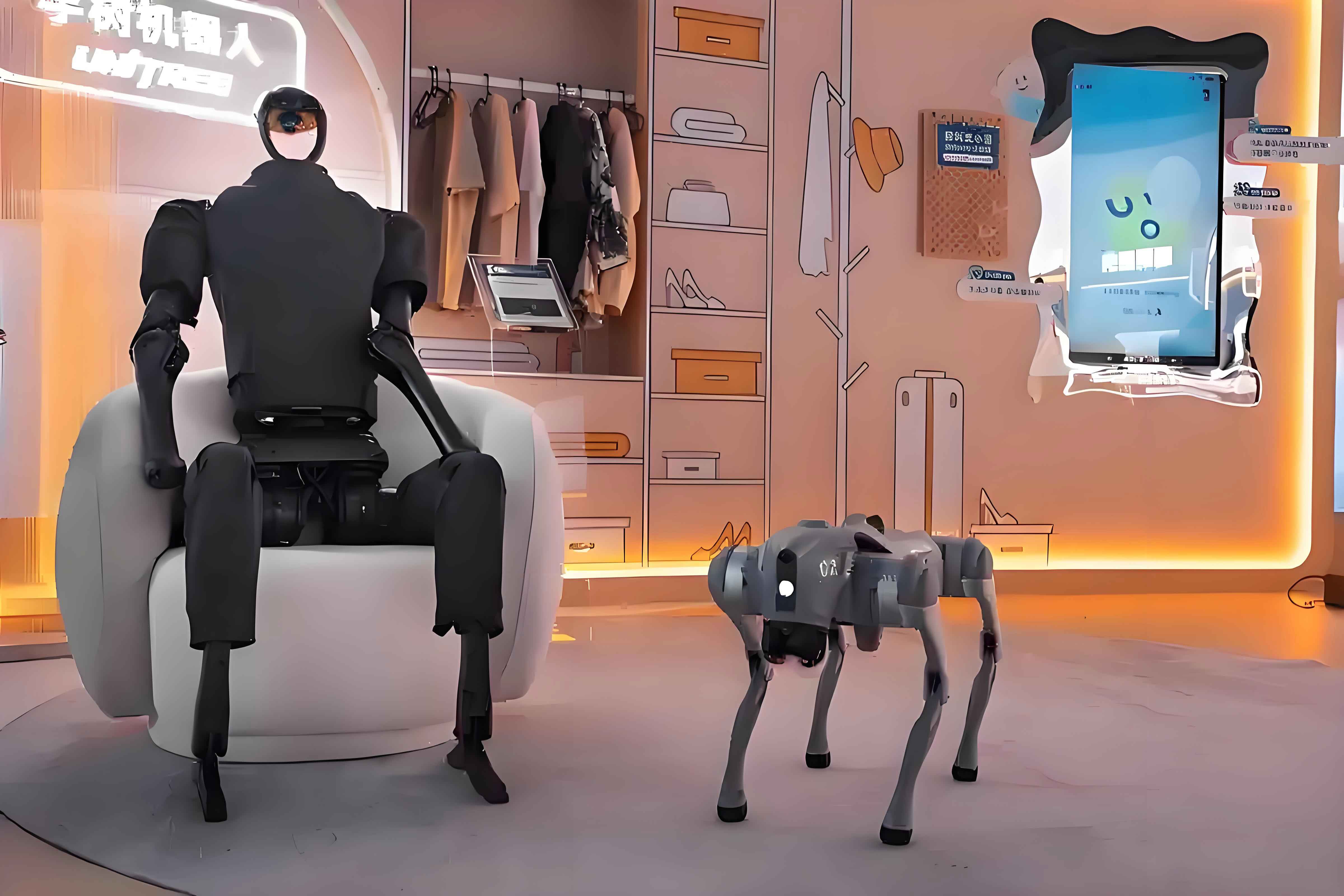
Figure 1: A typical scene of humanoid robots and robotic dogs.
3. Kinematics Modeling of the Humanoid Robot
Kinematics modeling is the foundation for gait planning and stability analysis. The biped humanoid robot has a tree-like structure with closed loops during the double-support phase and open chains during the single-support phase. To simplify the model, I assume that all links are rigid bodies and that the multiple axes of the same joint intersect at a single point. The upper body joints are kept locked during walking because they have little influence on the lower-limb motion. Therefore, the ROBOT-Ⅰ humanoid robot is abstracted as an 11-link mechanism: two legs (each with five links) plus a torso link. Each leg consists of a hip link, a thigh, a shank, and a foot. The right leg is modeled as an example.
3.1 Coordinate Frame Definition
I define a world coordinate frame \(O_w = (x_w, y_w, z_w)\) fixed on the ground, where \(x_w\) is the forward direction of the robot, \(z_w\) is vertical upward, and \(y_w\) is determined by the right-hand rule. A body coordinate frame \(O_0 = (x_0, y_0, z_0)\) is attached to the waist. Each link has a local coordinate frame. The DH parameters for the right leg are given in Table 3.
| Link \(i\) | \(a_{i-1}\) | \(\alpha_{i-1}\) | \(d_i\) | \(\theta_i\) |
|---|---|---|---|---|
| 1 | 0 | 0 | 0 | \(\theta_1\) |
| 2 | \(l_1\) | \(-90^\circ\) | 0 | \(\theta_2\) |
| 3 | \(l_2\) | 0 | 0 | \(\theta_3\) |
| 4 | \(l_3\) | 0 | 0 | \(\theta_4\) |
| 5 | \(l_4\) | \(90^\circ\) | 0 | \(\theta_5\) |
Table 3: DH parameters for the right leg of ROBOT-Ⅰ.
Here \(a_{i-1}\) is the link length, \(\alpha_{i-1}\) is the link twist, \(d_i\) is the link offset, and \(\theta_i\) is the joint angle. The transformation matrix from frame \(i-1\) to frame \(i\) is given by:
$$
T_i^{i-1} = \begin{bmatrix}
\cos\theta_i & -\sin\theta_i \cos\alpha_{i-1} & \sin\theta_i \sin\alpha_{i-1} & a_{i-1} \cos\theta_i \\
\sin\theta_i & \cos\theta_i \cos\alpha_{i-1} & -\cos\theta_i \sin\alpha_{i-1} & a_{i-1} \sin\theta_i \\
0 & \sin\alpha_{i-1} & \cos\alpha_{i-1} & d_i \\
0 & 0 & 0 & 1
\end{bmatrix}
$$
3.2 Forward Kinematics
The forward kinematics of the humanoid robot computes the pose of the foot (or any link) with respect to the reference frame as a function of the joint angles. For the right leg, the overall transformation from the waist frame to the foot frame is:
$$
T_5^0 = T_1^0 \, T_2^1 \, T_3^2 \, T_4^3 \, T_5^4
$$
Using the DH parameters, I obtain the individual transformation matrices:
$$
T_1^0 = \begin{bmatrix}
\cos\theta_1 & -\sin\theta_1 & 0 & 0 \\
\sin\theta_1 & \cos\theta_1 & 0 & 0 \\
0 & 0 & 1 & 0 \\
0 & 0 & 0 & 1
\end{bmatrix}, \quad
T_2^1 = \begin{bmatrix}
\cos\theta_2 & 0 & -\sin\theta_2 & l_1 \cos\theta_2 \\
\sin\theta_2 & 0 & \cos\theta_2 & l_1 \sin\theta_2 \\
0 & -1 & 0 & 0 \\
0 & 0 & 0 & 1
\end{bmatrix}
$$
$$
T_3^2 = \begin{bmatrix}
\cos\theta_3 & -\sin\theta_3 & 0 & l_2 \cos\theta_3 \\
\sin\theta_3 & \cos\theta_3 & 0 & l_2 \sin\theta_3 \\
0 & 0 & 1 & 0 \\
0 & 0 & 0 & 1
\end{bmatrix}, \quad
T_4^3 = \begin{bmatrix}
\cos\theta_4 & -\sin\theta_4 & 0 & l_3 \cos\theta_4 \\
\sin\theta_4 & \cos\theta_4 & 0 & l_3 \sin\theta_4 \\
0 & 0 & 1 & 0 \\
0 & 0 & 0 & 1
\end{bmatrix}
$$
$$
T_5^4 = \begin{bmatrix}
\cos\theta_5 & 0 & \sin\theta_5 & l_4 \cos\theta_5 \\
\sin\theta_5 & 0 & -\cos\theta_5 & l_4 \sin\theta_5 \\
0 & 1 & 0 & 0 \\
0 & 0 & 0 & 1
\end{bmatrix}
$$
By multiplying these matrices, the foot position and orientation in the waist frame are expressed as functions of the joint angles \(\theta_1,\dots,\theta_5\). This completes the forward kinematics solution.
3.3 Inverse Kinematics
The inverse kinematics problem is to find the joint angles given the desired position and orientation of the foot relative to the waist. This is essential for gait planning because the gait planner generates the foot and waist trajectories in Cartesian space, and the inverse kinematics maps them to joint space. I assume that during walking the torso remains horizontal and the foot is flat on the ground. Under these assumptions, the following constraints hold:
$$
\theta_1 + \theta_5 = 0
$$
$$
\theta_2 + \theta_3 + \theta_4 = 0
$$
Let the desired foot pose in the waist frame be:
$$
T_5^0 = \begin{bmatrix}
r_{11} & r_{12} & r_{13} & p_x \\
r_{21} & r_{22} & r_{23} & p_y \\
r_{31} & r_{32} & r_{33} & p_z \\
0 & 0 & 0 & 1
\end{bmatrix}
$$
By multiplying both sides of the equation with the inverse of \(T_1^0\), and using the equality of corresponding matrix elements, I can solve for the joint angles. For example, comparing the (2,1) elements yields:
$$
\theta_1 = \arctan\left(\frac{p_y}{p_x}\right)
$$
and subsequently \(\theta_5 = -\theta_1\). Further algebraic manipulation gives the remaining angles. The complete derivation is omitted here for brevity, but the result provides an analytic solution to the inverse kinematics of the ROBOT-Ⅰ humanoid robot. This solution is used in all gait planning experiments described below.
4. Gait Planning of the Biped Humanoid Robot
Gait planning is the process of generating the joint trajectories over time to achieve a desired walking motion. A good gait for a humanoid robot should satisfy several criteria: (1) the ZMP must remain inside the support polygon, (2) the joint trajectories should be smooth and continuous, (3) the gait should be energy efficient, and (4) the gait should be robust to external disturbances. In this section, I first introduce the ZMP stability criterion, then present a ZMP-based gait planner using the linear inverted pendulum model, and finally propose an improved optimization-based gait planner.
4.1 ZMP Stability Criterion
The Zero Moment Point (ZMP) is defined as the point on the ground where the resultant moment of the gravitational force, inertial force, and ground reaction force becomes zero. The ZMP stability criterion states that a biped humanoid robot is dynamically stable if and only if the ZMP lies inside the convex hull of the foot contact region. This criterion is widely used because it provides a necessary and sufficient condition for dynamic walking. The support polygon is the projection of the foot contact area on the ground. In the single-support phase, the support polygon is the area of the supporting foot. In the double-support phase, it is the convex hull of both feet.
The ZMP coordinates can be computed from the mass distribution and accelerations of the robot. For a multibody system, the ZMP is given by:
$$
p_x = \frac{\sum_{i} m_i (z_i \ddot{x}_i – x_i \ddot{z}_i + x_i g)}{\sum_{i} m_i (\ddot{z}_i + g)}
$$
$$
p_y = \frac{\sum_{i} m_i (z_i \ddot{y}_i – y_i \ddot{z}_i + y_i g)}{\sum_{i} m_i (\ddot{z}_i + g)}
$$
where \(m_i\) is the mass of the \(i\)-th link, \((x_i,y_i,z_i)\) is the position of its center of mass, and \(g\) is the gravitational acceleration. In the simplified linear inverted pendulum model, the ZMP is related to the center-of-mass (CoM) position by:
$$
p_x = x – \frac{z}{g} \ddot{x}
$$
$$
p_y = y – \frac{z}{g} \ddot{y}
$$
These equations form the basis of the gait planning method described next.
4.2 Gait Planning Using the Linear Inverted Pendulum Model
The linear inverted pendulum model (LIPM) abstracts the humanoid robot as a mass point located at the center of mass, connected to a massless telescopic leg that pivots at the foot contact point. The CoM is constrained to move on a horizontal plane at a constant height \(z_c\). In this case, the horizontal motion of the CoM is decoupled from the vertical motion and the dynamics become linear:
$$
\ddot{x} = \frac{g}{z_c} (x – p_x)
$$
$$
\ddot{y} = \frac{g}{z_c} (y – p_y)
$$
To generate a stable walking gait, the planner first specifies a desired ZMP trajectory that stays inside the support polygon. A common choice is to keep the ZMP at the center of the supporting foot during the single-support phase, and to move it linearly from the rear foot center to the front foot center during the double-support phase. Given the ZMP trajectory, the CoM trajectory can be obtained by solving the linear differential equations. A convenient method is to use the closed-form solution based on the “time-reversed” approach or to integrate the equations numerically with boundary conditions.
For the ROBOT-Ⅰ humanoid robot, I set the step length to 4 cm, the step period to 0.8 s, and the foot clearance to 1.5 cm. Using MATLAB, I computed the CoM trajectory and then used the inverse kinematics to obtain the joint angles for all six leg joints (three per leg). Figure 2 shows the joint angle profiles over one complete walking cycle. The angles are continuous and smooth, which is desirable for reducing wear and energy consumption. Figure 3 shows the joint angular velocities. The maximum angular velocity is approximately 3 rad/s, which is well within the capabilities of the servo motors.
| Joint | Max angle (degree) | Min angle (degree) | Max angular velocity (rad/s) |
|---|---|---|---|
| Left hip | 25.3 | -12.1 | 1.8 |
| Left knee | 48.2 | 2.4 | 2.7 |
| Left ankle | 18.6 | -15.3 | 1.9 |
| Right hip | 25.3 | -12.1 | 1.8 |
| Right knee | 48.2 | 2.4 | 2.7 |
| Right ankle | 18.6 | -15.3 | 1.9 |
Table 4: Joint angle ranges and maximum angular velocities in the planned gait.
I conducted walking experiments on the ROBOT-Ⅰ humanoid robot using this gait. The robot was able to walk forward, but it was not always stable; it often fell after a few steps, especially when starting or stopping. This indicates that the LIPM-based ZMP planning alone is insufficient for robust walking in practice due to model uncertainties and external disturbances. Therefore, an improved gait planning method is needed.
4.3 Improved Gait Planning Based on Optimization
Offline gait planners cannot modify the planning method itself during online operation. To overcome this limitation, I propose a new gait planning method that combines polynomial fitting of the ankle trajectory with a numerical optimization search for the hip trajectory. The method is designed to be sufficiently fast for online implementation.
First, the trajectory of the swing foot ankle is approximated by a polynomial. During the single-support phase, the supporting foot ankle is stationary, while the swing foot ankle moves from the rear position to the front position. I define the horizontal and vertical ankle positions as:
$$
x_h(t) = \sum_{i=0}^{5} a_i t^i
$$
$$
z_h(t) = \sum_{i=0}^{4} b_i t^i
$$
The coefficients are determined by the boundary conditions. Let \(t_{\text{begin}}\) be the lift-off time, \(t_{\text{high}}\) the time when the ankle reaches its highest point, and \(t_{\text{end}}\) the landing time. The constraints are:
$$
x_h(t_{\text{begin}}) = x_{\text{begin}}, \quad z_h(t_{\text{begin}}) = z_{\text{begin}}
$$
$$
x_h(t_{\text{high}}) = x_{\text{high}}, \quad z_h(t_{\text{high}}) = z_{\text{high}}
$$
$$
x_h(t_{\text{end}}) = x_{\text{end}}, \quad z_h(t_{\text{end}}) = z_{\text{end}}
$$
In addition, the vertical velocity at the beginning and at the end should be zero to reduce foot impact:
$$
\dot{z}_h(t_{\text{begin}}) = 0, \quad \dot{z}_h(t_{\text{end}}) = 0
$$
These constraints determine the polynomial coefficients. The ZMP trajectory is planned as described earlier. Next, the hip trajectory is searched using an optimization method. The hip position \((x_k, z_k)\) must satisfy the geometric constraints of the leg links. For each discrete time step \(t_j\), the robot configuration must produce a ZMP that is as close as possible to the desired ZMP. Thus the problem is formulated as:
$$
\min_{x_k(t_j), z_k(t_j)} \left\| p_x^{\text{actual}}(t_j) – p_x^{\text{planned}}(t_j) \right\|
$$
subject to:
$$
x_k^{\min} \le x_k(t_j) \le x_k^{\max}
$$
$$
z_k^{\min} \le z_k(t_j) \le z_k^{\max}
$$
The actual ZMP is computed from the link masses and accelerations. Since the ankle trajectory is known and the hip position is being optimized, the leg configuration is fully determined, and the ZMP can be calculated. I use a gradient descent algorithm to search for the hip position at each time step. In order to accelerate convergence, I modify the step size adaptively: when the gradient decreases slowly, the step size is increased to avoid becoming stuck in a slow convergence region. This modification is crucial for online planning because the search time is reduced significantly.
Figure 4 compares the planned ZMP trajectory with the actual ZMP obtained from the optimized hip trajectory. The error statistics are summarized in Table 5. The maximum error is 0.3236 cm, and the average error is 0.1651 cm. These values are acceptable for the 4 cm step length, and the small error confirms that the optimization-based gait planner can generate a hip trajectory that closely tracks the desired ZMP.
| Error metric | Value (cm) |
|---|---|
| Maximum error | 0.3236 |
| Minimum error | 0.0094 |
| Average error | 0.1651 |
| Variance | 0.0110 |
Table 5: ZMP tracking error of the optimization-based gait planner.
The experimental results show that the optimization-based method produces a stable gait, and the search speed is acceptable for online implementation. The improved step size control reduces the computation time by about 30% compared to the standard gradient descent method.
5. Stability Control Based on Attitude Detection
Even with a well-planned gait, the actual motion of the humanoid robot deviates from the desired motion due to model uncertainties, joint elasticity, sensor noise, and external disturbances. To achieve robust walking, the robot must sense its state and adjust its motion accordingly. In this section, I describe the attitude estimation and stability feedback control framework implemented on ROBOT-Ⅰ.
5.1 Attitude Representation Using Euler Angles and Quaternions
The orientation of the humanoid robot torso relative to the world frame can be represented by three Euler angles: yaw \(\psi\), pitch \(\theta\), and roll \(\phi\). The rotation matrix from the body frame to the world frame is:
$$
R = R_z(\psi) R_y(\theta) R_x(\phi)
$$
where
$$
R_z(\psi) = \begin{bmatrix}
\cos\psi & -\sin\psi & 0 \\
\sin\psi & \cos\psi & 0 \\
0 & 0 & 1
\end{bmatrix}
$$
$$
R_y(\theta) = \begin{bmatrix}
\cos\theta & 0 & \sin\theta \\
0 & 1 & 0 \\
-\sin\theta & 0 & \cos\theta
\end{bmatrix}
$$
$$
R_x(\phi) = \begin{bmatrix}
1 & 0 & 0 \\
0 & \cos\phi & -\sin\phi \\
0 & \sin\phi & \cos\phi
\end{bmatrix}
$$
Although Euler angles are intuitive, they suffer from singularities and require many trigonometric computations. For real-time control, I use quaternions. A quaternion \(q = (q_0, q_1, q_2, q_3)\) represents a rotation by an angle \(\Omega\) about a unit vector \(e = (e_x, e_y, e_z)\):
$$
q = \begin{bmatrix}
\cos(\Omega/2) \\
e_x \sin(\Omega/2) \\
e_y \sin(\Omega/2) \\
e_z \sin(\Omega/2)
\end{bmatrix}
$$
The rotation matrix in terms of quaternions is:
$$
R(q) = \begin{bmatrix}
1 – 2(q_2^2 + q_3^2) & 2(q_1 q_2 – q_0 q_3) & 2(q_1 q_3 + q_0 q_2) \\
2(q_1 q_2 + q_0 q_3) & 1 – 2(q_1^2 + q_3^2) & 2(q_2 q_3 – q_0 q_1) \\
2(q_1 q_3 – q_0 q_2) & 2(q_2 q_3 + q_0 q_1) & 1 – 2(q_1^2 + q_2^2)
\end{bmatrix}
$$
The quaternion dynamic equation is:
$$
\dot{q} = \frac{1}{2} \begin{bmatrix}
0 & -\omega_x & -\omega_y & -\omega_z \\
\omega_x & 0 & \omega_z & -\omega_y \\
\omega_y & -\omega_z & 0 & \omega_x \\
\omega_z & \omega_y & -\omega_x & 0
\end{bmatrix} q
$$
where \((\omega_x, \omega_y, \omega_z)\) is the angular velocity measured by the gyroscope. I integrate this equation using a first-order Runge-Kutta method. The gyroscope drift is compensated by the accelerometer data through a complementary filter. This approach is computationally efficient and suitable for the LPC1768 microcontroller.
5.2 Torso Attitude Controller
The torso of a humanoid robot should remain as close to the desired upright orientation as possible. If the torso leans too much, the gravitational torque about the support foot becomes large and the robot may fall. The hip joint of the supporting leg is the most effective joint for correcting torso orientation. The torso attitude controller adjusts the hip joint angle according to the following law:
$$
\theta_{\text{hip, correction}} = K_{p1} (\theta_{\text{desired}} – \theta_{\text{actual}}) + K_{d1} (\dot{\theta}_{\text{desired}} – \dot{\theta}_{\text{actual}})
$$
where \(K_{p1}\) and \(K_{d1}\) are the proportional and derivative gains. The controller is simple but effective, as demonstrated by the experimental results below.
5.3 ZMP Compensator
Although the ROBOT-Ⅰ humanoid robot does not have force sensors to measure the actual ZMP, the ZMP can be estimated from the joint angles and the torso attitude using the dynamic model. The ZMP compensator adjusts the ankle joint of the supporting foot to reduce the error between the actual and desired ZMP. The control law is:
$$
\theta_{\text{ankle, correction}} = K_{p2} (p_{x}^{\text{desired}} – p_{x}^{\text{actual}}) + K_{d2} (\dot{p}_{x}^{\text{desired}} – \dot{p}_{x}^{\text{actual}})
$$
A similar law applies for the \(y\)-direction. The ZMP compensator works in coordination with the torso controller. The overall feedback control structure is shown in Figure 5.
5.4 Experimental Evaluation
I performed walking experiments on the ROBOT-Ⅰ humanoid robot with and without the stability feedback control. The robot was commanded to walk on a flat ground surface. The torso pitch angle was recorded during walking. Table 6 shows the statistics of the pitch angle error with respect to the desired vertical orientation. Without control, the maximum error was 0.2156 rad, the mean error was 0.0762 rad, and the variance was 0.0043. With the torso attitude controller, the maximum error was reduced to 0.0702 rad, the mean error to 0.0241 rad, and the variance to 0.0003. These results demonstrate that the torso controller significantly improves the torso stability.
| Statistic | Without control | With torso control |
|---|---|---|
| Maximum error (rad) | 0.2156 | 0.0702 |
| Mean error (rad) | 0.0762 | 0.0241 |
| Variance (rad²) | 0.0043 | 0.0003 |
Table 6: Torso pitch angle error statistics before and after control.
Table 7 shows the ZMP tracking error in the x and y directions. In the x direction, the maximum error was reduced from 1.2000 cm to 1.0000 cm, and the mean error from 0.4800 cm to 0.2900 cm. In the y direction, the maximum error was reduced from 3.8000 cm to 2.5000 cm, demonstrating that the ZMP compensator improves the walking balance.
| Direction | Statistic | Before compensation | After compensation |
|---|---|---|---|
| x | Max (cm) | 1.2000 | 1.0000 |
| x | Mean (cm) | 0.4800 | 0.2900 |
| x | Variance (cm²) | 0.1640 | 0.1277 |
| y | Max (cm) | 3.8000 | 2.5000 |
| y | Mean (cm) | 1.0200 | 0.6400 |
| y | Variance (cm²) | 1.1796 | 0.9804 |
Table 7: ZMP error statistics before and after compensation.
In disturbance rejection experiments, I gently pushed the robot while it was walking. With the feedback controller, the robot was able to recover its balance automatically by adjusting its steps. When a large disturbance was applied, the robot executed a protective fall movement to avoid damage, and then it stood up again. These experiments confirm that the attitude-based stability feedback control makes the humanoid robot much more robust to unknown disturbances.
6. Conclusion
In this thesis, I have presented a comprehensive study of gait planning and stability control for the ROBOT-Ⅰ biped humanoid robot. The main conclusions are as follows.
First, I established a kinematics model for the humanoid robot using the DH convention. The forward and inverse kinematics solutions provide the mapping between joint space and Cartesian space, which is fundamental for all subsequent motion planning.
Second, I implemented a ZMP-based gait planner using a three-dimensional linear inverted pendulum model. The planned joint trajectories are smooth and continuous, and the robot can walk forward using this gait. However, the walking is not sufficiently stable in practice due to model uncertainties.
Third, I proposed an improved optimization-based gait planning method. The ankle trajectory is generated by polynomial fitting, and the hip trajectory is obtained by minimizing the ZMP tracking error using a fast gradient search with adaptive step size. The simulation and experimental results show that this method reduces the ZMP error significantly and has the potential for online planning.
Finally, I designed a stability feedback controller based on attitude detection. The IMU sensor (MPU6050) provides the angular velocity and acceleration of the torso. A quaternion-based attitude estimation algorithm computes the torso orientation in real time. A torso attitude controller and a ZMP compensator correct the joint trajectories online. Experiments demonstrate that the feedback control greatly improves the walking stability and disturbance rejection capability of the humanoid robot.
The research presented in this thesis contributes to the field of biped humanoid robots by providing a complete framework from mechanical design to model-based gait planning and sensor-based stability control. Future work will focus on improving the optimization-based planner to handle uneven terrain, stairs, and obstacles, as well as incorporating visual sensors for autonomous navigation. The humanoid robot remains a fascinating and challenging platform, and I believe that its potential in real-world applications is enormous.