
In the field of robotics and precision engineering, the demand for high-performance force sensing has grown significantly, particularly in applications such as rocket engine testing, wind tunnel experiments, and heavy-duty industrial automation. A six-axis force sensor is capable of measuring all six components of force and torque, making it indispensable for tasks requiring precise force feedback and control. Traditional six-axis force sensors often face challenges in heavy-load scenarios due to limitations in stiffness, size, and accuracy. To address these issues, a heavy-duty parallel six-axis force sensor with a hybrid branch structure has been developed. This design incorporates both measuring branches and load-bearing branches, enhancing the sensor’s stiffness and load capacity while maintaining a compact form factor. This article explores the structural characteristics, measurement principles, and static calibration of this sensor, with a focus on improving accuracy through advanced calibration algorithms.
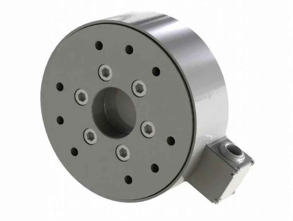
The six-axis force sensor is based on a parallel mechanism, which offers advantages such as high stiffness, stability, and no error accumulation. The proposed sensor features an inner ring as the measuring platform and an outer ring as the fixed platform, connected by eight measuring branches and four load-bearing branches. The measuring branches utilize strain gauges to detect deformations under load, converting mechanical strain into voltage signals. These signals are then processed to determine the applied forces and torques. The load-bearing branches, designed as rectangular beams, increase the overall stiffness of the sensor, allowing it to handle heavy loads without compromising sensitivity. The sensor is manufactured using titanium alloy powder and 3D printing technology, resulting in a compact size of Ø180 mm × 17 mm height. The measuring range of the sensor is summarized in Table 1.
| Force Component | Range |
|---|---|
| F_x | ±5 kN |
| F_y | ±5 kN |
| F_z | ±3 kN |
| M_x | ±50 N·m |
| M_y | ±50 N·m |
| M_z | ±90 N·m |
The measurement principle of the six-axis force sensor relies on the static equilibrium of spatial force systems. When an external force or torque is applied to the sensor’s platform, the measuring branches experience deformations, which are detected by strain gauges. The voltage signals from these strain gauges are amplified, filtered, and converted to digital signals for processing. The relationship between the applied six-dimensional force vector and the output voltage signals can be expressed as:
$$ \mathbf{F}_{6 \times 1} = \mathbf{G}_{6 \times 8} \mathbf{U}_{8 \times 1} $$
where \(\mathbf{F}_{6 \times 1}\) is the applied force and torque vector, \(\mathbf{G}_{6 \times 8}\) is the calibration matrix that maps the voltage signals to the forces, and \(\mathbf{U}_{8 \times 1}\) is the voltage output vector from the eight measuring branches. Solving for the calibration matrix \(\mathbf{G}\) is a key step in the sensor’s calibration process. However, due to manufacturing errors, environmental factors, and inter-dimensional coupling, the sensor’s output may deviate from the ideal linear relationship. Therefore, advanced calibration algorithms are necessary to improve accuracy.
Static calibration is crucial for ensuring the precision of the six-axis force sensor. The calibration process involves applying known forces and torques to the sensor and recording the corresponding voltage outputs. A calibration system typically includes hardware components such as a signal acquisition box, a six-axis force measurement table, loading devices (e.g., weights and jacks), and software for data processing. The six-axis force measurement table used in this study has an accuracy of 0.5% for force and 1% for torque, with a measuring range as shown in Table 2.
| Force Component | Range |
|---|---|
| F_x | -10 to +10 kN |
| F_y | -10 to +10 kN |
| F_z | -30 to +30 kN |
| M_x | -100 to +100 N·m |
| M_y | -100 to +100 N·m |
| M_z | -100 to +100 N·m |
The calibration procedure involves loading the sensor in each direction (Fx, Fy, Fz, Mx, My, Mz) at multiple points within the measuring range. For force components Fx and Fy, a hydraulic jack is used to apply loads, while for Fz, weights are placed on a loading tray. Torque components Mx and My are generated by applying forces at a known distance from the sensor’s center, and Mz is applied using a jack to create a moment arm. The voltage signals are recorded at each loading point, and the data is used to compute the calibration matrix.
To evaluate the performance of the six-axis force sensor, the calibration error matrix is defined as:
$$ \boldsymbol{\xi} = (\mathbf{F}_r – \mathbf{F}_c) \mathbf{F}_{fs}^{-1} $$
where \(\mathbf{F}_r\) is the actual applied force matrix, \(\mathbf{F}_c\) is the calculated force matrix from the calibration data, and \(\mathbf{F}_{fs}\) is a diagonal matrix containing the full-scale values of each force and torque component. The diagonal elements of \(\boldsymbol{\xi}\) represent the nonlinear errors in each direction, while the off-diagonal elements indicate the inter-dimensional coupling errors. The goal of calibration is to minimize both types of errors.
Several calibration algorithms are employed to improve the accuracy of the six-axis force sensor. The least squares method is a common approach for linear systems. Given the voltage output matrix \(\mathbf{U}\) and the applied force matrix \(\mathbf{F}\), the calibration matrix \(\mathbf{G}\) can be computed as:
$$ \mathbf{G}_{6 \times 8} = \mathbf{F}_{6 \times n} \mathbf{U}_{8 \times n}^T (\mathbf{U}_{8 \times n} \mathbf{U}_{8 \times n}^T)^{-1} $$
where \(n\) is the number of calibration data points. However, the least squares method may not adequately address nonlinearities and coupling effects in the sensor. Therefore, nonlinear calibration algorithms such as the backpropagation (BP) neural network are used. The BP neural network models the relationship between the voltage inputs and force outputs through multiple layers. The network structure includes an input layer with eight nodes (corresponding to the voltage signals), a hidden layer with a variable number of nodes, and an output layer with six nodes (corresponding to the force and torque components). The hidden layer uses a hyperbolic tangent activation function, while the output layer uses a linear activation function. The network is trained using the Levenberg-Marquardt algorithm.
The performance of the BP neural network depends on the number of hidden nodes. Through experimentation, it was found that 14 hidden nodes yield the best results for this six-axis force sensor. The BP neural network algorithm reduces both nonlinear and coupling errors compared to the least squares method. However, the BP neural network can be prone to local minima during training. To address this, an optimized BP neural network based on the artificial fish swarm algorithm (AFSA) is proposed. The AFSA optimizes the initial weights and thresholds of the BP neural network by simulating the behaviors of fish swarms, such as foraging, swarming, and following. This optimization helps the network converge to a global optimum and improves stability.
The artificial fish swarm algorithm involves the following steps: First, parameters such as the number of artificial fish, visual step coefficient, and maximum iterations are set. Each artificial fish represents a set of weights and thresholds for the BP neural network. The distance between two artificial fish is calculated based on the Euclidean distance of their weight and threshold vectors. The artificial fish then perform behaviors to improve their position, and the best solution is used to initialize the BP neural network. This hybrid approach combines the global search capability of AFSA with the local search ability of BP, resulting in a more robust calibration algorithm.
Experimental results from the static calibration of the six-axis force sensor are presented below. The calibration data was divided into two sets: one for training (82 data points) and one for testing (41 data points). The least squares method was applied to the training data, resulting in the following calibration matrix:
$$ \mathbf{G}_c = \begin{bmatrix}
0.9858 & 0.8677 & 0.9724 & 1.0733 & -1.0339 & -0.9255 & 1.0964 & 0.9422 \\
-0.0870 & -0.2020 & 0.5582 & 0.4089 & 1.9098 & 2.0055 & 1.3989 & 1.5189 \\
0.8903 & 0.0929 & 0.0360 & 0.7883 & 0.9142 & 0.0424 & -0.6822 & 0.0304 \\
-0.0345 & -0.0177 & 0.0056 & 0.0195 & 0.0414 & 0.0252 & 0.0529 & 0.0358 \\
-0.0311 & -0.0118 & -0.0258 & -0.0474 & 0.0580 & 0.0300 & -0.0413 & -0.0144 \\
-0.0702 & -0.0018 & -0.0404 & 0.0296 & -0.0863 & -0.0089 & -0.0272 & 0.0440
\end{bmatrix} $$
The corresponding calibration error matrix for the test data was:
$$ \boldsymbol{\xi}_c = \begin{bmatrix}
0.0265 & 0.0113 & 0.0066 & 0.0029 & 0.0044 & 0.0208 \\
0.0306 & 0.0248 & 0.0099 & 0.0043 & 0.0012 & 0.0257 \\
0.0536 & 0.0572 & 0.0268 & 0.0294 & 0.0153 & 0.0186 \\
0.0655 & 0.1057 & 0.0170 & 0.0675 & 0.0169 & 0.0606 \\
0.0931 & 0.0283 & 0.0535 & 0.0284 & 0.0423 & 0.0306 \\
0.0978 & 0.1032 & 0.0471 & 0.0311 & 0.0149 & 0.0498
\end{bmatrix} $$
This error matrix shows a maximum nonlinear error of 6.75% and a maximum coupling error of 10.57%. The BP neural network with 14 hidden nodes produced a better calibration error matrix:
$$ \boldsymbol{\xi}_{BP} = \begin{bmatrix}
0.0045 & 0.0052 & 0.0040 & 0.0015 & 0.0025 & 0.0033 \\
0.0037 & 0.0038 & 0.0035 & 0.0021 & 0.0028 & 0.0039 \\
0.0020 & 0.0028 & 0.0028 & 0.0012 & 0.0013 & 0.0045 \\
0.0044 & 0.0068 & 0.0093 & 0.0046 & 0.0048 & 0.0090 \\
0.0049 & 0.0033 & 0.0086 & 0.0035 & 0.0076 & 0.0038 \\
0.0088 & 0.0066 & 0.0029 & 0.0018 & 0.0037 & 0.0065
\end{bmatrix} $$
Here, the maximum nonlinear error was 0.76% and the maximum coupling error was 0.93%. The optimized BP neural network with AFSA further improved the results, yielding the following error matrix:
$$ \boldsymbol{\xi}_{OBP} = \begin{bmatrix}
0.0039 & 0.0030 & 0.0045 & 0.0029 & 0.0023 & 0.0027 \\
0.0046 & 0.0043 & 0.0027 & 0.0018 & 0.0015 & 0.0030 \\
0.0033 & 0.0019 & 0.0019 & 0.0017 & 0.0015 & 0.0020 \\
0.0035 & 0.0087 & 0.0084 & 0.0049 & 0.0048 & 0.0055 \\
0.0053 & 0.0027 & 0.0070 & 0.0032 & 0.0042 & 0.0047 \\
0.0090 & 0.0036 & 0.0053 & 0.0020 & 0.0059 & 0.0044
\end{bmatrix} $$
This represents a maximum nonlinear error of 0.49% and a maximum coupling error of 0.9%. A comparison of the accuracy for each force component using different methods is summarized in Table 3.
| Method | F_x (%) | F_y (%) | F_z (%) | M_x (%) | M_y (%) | M_z (%) |
|---|---|---|---|---|---|---|
| Least Squares | 2.65 | 2.48 | 2.68 | 6.75 | 4.23 | 4.98 |
| BP Neural Network | 0.53 | 0.45 | 0.30 | 0.45 | 0.61 | 0.53 |
| Optimized BP with AFSA | 0.39 | 0.43 | 0.19 | 0.49 | 0.42 | 0.44 |
The results demonstrate that the BP neural network algorithms significantly outperform the least squares method in reducing both nonlinear and coupling errors. The optimized BP neural network with AFSA provides the best performance, with stable results and a reduced tendency to fall into local minima. This makes it a reliable choice for calibrating heavy-duty six-axis force sensors.
In conclusion, the heavy-duty parallel six-axis force sensor with a hybrid branch structure offers a compact and robust solution for high-load applications. The integration of measuring and load-bearing branches enhances stiffness and load capacity without sacrificing sensitivity. Static calibration using advanced algorithms like the BP neural network and its optimized version with AFSA effectively addresses nonlinearities and inter-dimensional coupling, resulting in high accuracy. The experimental validation confirms the superiority of these methods over traditional least squares, providing a foundation for future improvements in six-axis force sensor technology. This research contributes to the development of reliable force sensing systems for demanding industrial and scientific applications.