
In recent years, the development of humanoid robots has drawn significant attention to their autonomous locomotion capabilities in complex terrains. Unlike wheeled robots or drones, humanoid robots rely solely on two feet for support, which introduces stringent requirements for real-time perception and planning. In particular, the ability to construct a reliable representation of the environment and to generate safe footstep sequences is essential for tasks such as stair climbing and navigation over uneven surfaces. In this work, we focus on the key problems of terrain mapping and foothold planning for humanoid robots operating in complex environments. We propose a real-time 3D polygonal mapping framework that leverages GPU acceleration for depth image filtering and plane extraction, and we introduce a guided RRT* algorithm based on a neighbor-guided topology map to efficiently search for feasible footstep sequences. Extensive experiments on stair-like terrains demonstrate the effectiveness and practicality of the proposed methods.
1. Introduction
Humanoid robots are expected to operate in environments designed for humans, such as staircases, rubble, and other unstructured terrains. To achieve autonomous walking in such environments, a humanoid robot must be able to: (1) estimate its own pose accurately, (2) build a terrain map that contains sufficient geometric information for foot placement, and (3) plan a sequence of foot placements that satisfies both kinematic and dynamic constraints. Traditional approaches often rely on pre-modeled environments or simple elevation maps, which are insufficient for the high precision required by bipedal locomotion.
In this paper, we address these challenges by proposing an integrated pipeline for complex terrain walking. Our main contributions are summarized as follows:
- We systematically review the perception and planning framework for humanoid robots in complex terrains, covering pose estimation, terrain representation, and footstep planning methods.
- We design a real-time 3D polygonal terrain mapping algorithm that achieves high plane extraction accuracy and efficiency by using GPU-accelerated anisotropic diffusion filtering and RANSAC plane fitting.
- We propose a neighbor-guided topology map and integrate it with an improved RRT* algorithm to overcome the blind search problem in complex stair environments, significantly improving search efficiency and success rate.
The remainder of this paper is organized as follows. Section 2 reviews the related work. Section 3 describes the proposed polygonal mapping method. Section 4 presents the footstep planning algorithm. Section 5 reports experimental results on both simulated and real stair scenarios. Finally, Section 6 concludes the paper.
2. Related Work
2.1 Pose Estimation for Humanoid Robots
Accurate pose estimation is the foundation of terrain mapping and navigation. Several categories of methods exist, including leg odometry, visual odometry, and LiDAR odometry. Leg odometry uses forward kinematics based on joint encoders and a known contact state. For a robot with 12-DOF legs, the forward kinematics can be computed using the product of exponentials formula. Let each joint have a rotation axis vector \(a_i\) and a position vector \(b_i\) relative to its parent link. The homogeneous transformation of link \(j\) with respect to the base is:
$$ T_{i}^{j} = T_{i} \cdot \begin{bmatrix} e^{\hat{a}_j q_j} & b_j \\ 0 & 1 \end{bmatrix} $$
where \(q_j\) is the joint angle and \(\hat{a}_j\) is the skew-symmetric matrix of \(a_j\). By assuming the supporting foot is fixed on the ground, the body pose can be estimated recursively. However, leg odometry suffers from drift due to foot slippage and link deformation.
Visual odometry (VO) estimates motion from consecutive camera images. Feature-based methods, such as ORB-SLAM, extract keypoints and compute descriptors, then solve the perspective-n-point (PnP) problem to minimize the reprojection error. The reprojection error for a 3D point \(P\) projected into image \(I_2\) is:
$$ e = \sum_{i} \left\| p_i – K \exp(\hat{\xi}) P_i \right\|^2 $$
where \(K\) is the camera intrinsic matrix, \(\xi\) is the Lie algebra of the pose, and \(p_i\) is the observed pixel coordinate. Visual-inertial fusion (e.g., VINS-Fusion) further tightly couples IMU measurements with visual observations to improve robustness.
LiDAR odometry, such as LOAM and LIO-SAM, extracts edge and planar features from point clouds and registers consecutive scans. The residual for a planar feature point \(p_i\) to a corresponding planar patch is:
$$ d_{\perp} = \frac{|(p_i – p_a) \cdot n|}{|n|} $$
where \(p_a\) is a point on the plane and \(n\) is the plane normal. LiDAR methods provide accurate local estimates but require sufficient geometric features.
2.2 Point Cloud Filtering and Plane Extraction
Terrain mapping often relies on depth sensors that produce noisy point clouds. For depth images, edge-preserving filters such as bilateral filtering and guided filtering are widely used. The bilateral filter output is given by:
$$ I_{\text{filtered}}(x) = \frac{1}{W_p} \sum_{x_i \in \Omega} f_p(\|I(x_i)-I(x)\|) \, g_s(\|x_i-x\|) \, I(x_i) $$
with \(W_p\) as the normalization factor. Guided filtering assumes a local linear model between the guidance image \(I\) and the output \(q\):
$$ q_i = a_k I_i + b_k, \quad \forall i \in \omega_k $$
where \(a_k, b_k\) are constant coefficients computed by minimizing the cost function in a window.
Anisotropic diffusion filtering is another effective edge-preserving approach. The diffusion process is modeled by:
$$ \frac{\partial I}{\partial t} = \nabla \cdot (c(\nabla I) \nabla I) $$
with \(c(\nabla I) = \exp(-(\|\nabla I\|/k)^2)\) so that edges are preserved while flat regions are smoothed.
For plane extraction, RANSAC is a robust algorithm that iteratively samples three points to generate a plane hypothesis and then counts the inliers within a distance threshold. The plane equation is:
$$ ax + by + cz + d = 0 $$
GPU acceleration can parallelize inlier counting across many random hypotheses, greatly increasing speed. Region growing methods, on the other hand, use normal vectors and spatial proximity to merge points into planar segments.
2.3 Terrain Map Representations
Common terrain representations include octree maps, elevation maps, and polygonal maps. Octree maps store occupancy probabilities in a hierarchical voxel structure, providing memory efficiency for large environments. Elevation maps encode the height of the terrain in a regular 2.5D grid, which is suitable for non-rigid terrain but lacks explicit planar information. Polygonal maps represent terrain as a set of planar polygons, which aligns well with the foot placement requirement of humanoid robots. Each polygon encodes the plane equation and the boundary. Polygonal maps are compact and directly usable for footstep planning.
2.4 Footstep Planning Algorithms
Footstep planning searches for a sequence of foot placements from the current stance to a goal. A* is a classic graph-search algorithm that works on a discretized set of footstep states. The cost function is \(f(n) = g(n) + h(n)\), where \(g(n)\) is the cumulative cost from the start and \(h(n)\) is a heuristic estimate to the goal. A* is efficient in structured environments but may suffer from large computation in unstructured scenes.
RRT* is a sampling-based planner that incrementally builds a tree of feasible footholds. It randomly samples a state, connects it to the nearest node, and rewires the tree to asymptotically guarantee optimality. However, uniform sampling is often inefficient in complex stair environments because many samples are wasted in unreachable regions. In this paper, we improve RRT* by using a topology-guided sampling strategy.
3. Real-Time 3D Polygonal Terrain Mapping
We propose a mapping algorithm that receives depth images synchronized with pose estimates from a visual-inertial odometry and produces a global 3D polygonal map. The overall pipeline is shown in the following figure (the figure is a representative illustration of the system concept).
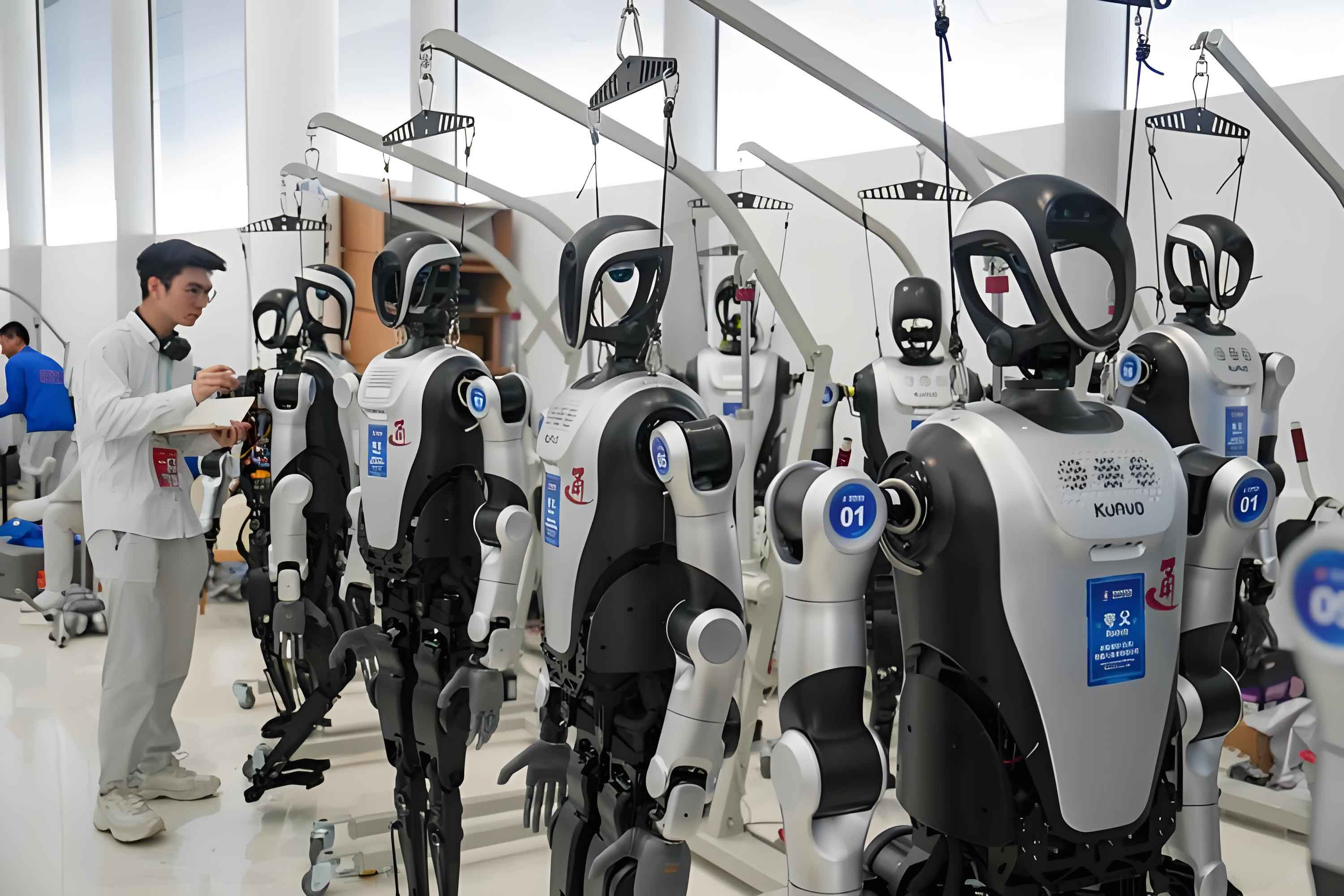
The algorithm consists of three main stages: depth image processing, plane extraction and fitting, and incremental map management.
3.1 Depth Image Processing
To reduce sensor noise while preserving edges, we apply anisotropic diffusion filtering on the GPU. The update rule for each pixel \(p\) at iteration \(t\) is:
$$ I_{p,t+1} = I_{p,t} + \gamma \sum_{q \in N(p)} c(\nabla I_{p,t}) \nabla I_{p,q,t} $$
where \(\gamma\) is the step size and \(N(p)\) is the four-connected neighborhood. In our implementation, we set \(k=134\), \(\gamma=0.2\), and perform 60 iterations for high-quality smoothing.
After filtering, we compute the normal vector for each pixel using the gradients along the horizontal and vertical directions. Given the depth \(Z\) at pixel \((x,y)\), the 3D point coordinates are:
$$ X = \frac{(u – c_x) Z}{f_x}, \quad Y = \frac{(v – c_y) Z}{f_y}, \quad Z = Z $$
From the gradients \(G_x = \partial Z / \partial u\) and \(G_y = \partial Z / \partial y\), the normal vector \(n_p\) is computed as:
$$ n_p = -\text{normalize}(K^{-1} [G_x, G_y, 1]^T) $$
where \(K\) is the camera intrinsic matrix. Figure 3.3 in the original work demonstrated that the filtered depth image yields much cleaner normal maps.
3.2 Plane Extraction and Fitting
We use two steps to extract planes from the normal image. First, we detect edges using the Canny algorithm on the normal image. The resulting binary edge image is then processed to extract contours, which are simplified using convex hull algorithms. Each convex polygon corresponds to a candidate planar region. For every candidate, we apply a GPU-accelerated RANSAC algorithm to fit the plane model. To speed up the process, we parallelize the RANSAC iterations on the GPU. For each hypothesis, we compute the distance from every point to the plane:
$$ \rho(p,\pi) = \frac{|a x_p + b y_p + c z_p + d|}{\sqrt{a^2 + b^2 + c^2}} $$
Points with \(\rho < \tau\) are considered inliers. The hypothesis with the largest number of inliers is refined using all inliers. The GPU parallelization significantly reduces the processing time, allowing the algorithm to run at more than 30 Hz for 640×480 depth images.
Table 3-1 reports the quantitative results of single-frame extraction on a standard stair model. We evaluated the average angle deviation \(\alpha\), the standard deviation of the normal direction \(\sigma_\alpha\), the intersection-over-union (IOU) between the extracted polygon and ground truth, and the height error \(\Delta d\).
| Trial | \(\alpha\) (deg) | \(\sigma_\alpha\) (deg) | IOU | \(\Delta d\) (mm) | \(\sigma_{\Delta d}\) (mm) |
|---|---|---|---|---|---|
| 1 | 2.22 | 0.459 | 0.936 | 3.2 | 1.51 |
| 2 | 2.15 | 0.410 | 0.922 | 1.8 | 1.72 |
| 3 | 2.22 | 0.453 | 0.940 | 1.3 | 2.03 |
Compared with the PPRCoRT method, our approach achieves better IOU and height accuracy while maintaining a comparable normal consistency. Table 3-2 summarizes the comparison:
| Method | \(\Delta d\) (mm) | \(\sigma_{\Delta d}\) (mm) | \(\sigma_\alpha\) (deg) | IOU | Time (ms) |
|---|---|---|---|---|---|
| PPRCoRT | 20.2 | 5.33 | 0.48 | 0.88 | 24 |
| Ours | 2.1 | 1.75 | 0.44 | 0.93 | 7.5 |
3.3 Incremental Map Management
To create a global map, we need to merge local frame polygons into a common frame. We use a visual-inertial odometry (VINS-Fusion) as the pose source. Because the depth camera has a limited field of view, the same terrain region may be observed from multiple viewpoints. The map manager integrates these measurements and updates the global polygonal representation.
The merging process first transforms the local polygon vertices into the global frame using the current pose. Then, for each new polygon, we search for an existing polygon in the map that overlaps in the XY projection. If the height difference and normal angle are below thresholds, we merge them by computing the convex hull of the union of their vertices:
$$ V_{\text{merged}} = \text{ConvexHull}(V_A \cup V_B) $$
To compensate for vertical drift, we design a Kalman filter that estimates the height offset between successive frames. The state model assumes constant drift:
$$ x_k = x_{k-1} + w_k, \quad w_k \sim \mathcal{N}(0, \sigma_p^2) $$
The measurement is the height difference between matched polygons:
$$ z_k = h_{\text{map}} – h_{\text{new}} + v_k, \quad v_k \sim \mathcal{N}(0, \sigma_m^2) $$
The Kalman gain \(K_k\) and update equations are:
$$ K_k = \frac{P_{k|k-1}}{P_{k|k-1} + \sigma_m^2}, \quad \hat{x}_k = \hat{x}_{k-1} + K_k (z_k – \hat{x}_{k-1}) $$
$$ P_{k} = (1 – K_k) P_{k|k-1} $$
Here, \(P\) is the error covariance. We then correct all polygon heights in the current frame using the estimated drift. This avoids cumulative vertical errors during long traversals.
3.4 Global Mapping Results
We performed global mapping experiments in two indoor stair environments: a straight staircase and a spiral staircase. The sensor setup consisted of a RealSense D435i for visual-inertial odometry and a RealSense L515 for terrain sensing. Figure 3.6 in the original work showed the constructed polygonal map with the VO trajectory.
We compared our polygonal map with the open-source elevation mapping library (EM_cupy). Table 3-3 presents the statistical results on a straight staircase.
| Method | Map type | \(\alpha\) (deg) | \(\sigma_\alpha\) (deg) | IOU | \(\Delta d\) (mm) |
|---|---|---|---|---|---|
| EM_cupy | grid (1 cm) | 8.17 | 4.39 | 0.61 | 5.7 |
| Ours | polygon | 4.74 | 1.02 | 0.96 | 5.3 |
The polygonal representation is not limited by a fixed resolution and provides cleaner plane regions. Moreover, our method automatically excludes non-planar areas, such as the robot’s own body parts that may appear in the field of view, whereas the elevation map is disturbed by dynamic obstacles and produces false bumps.
4. Footstep Planning with Guided RRT*
After obtaining the global polygonal map, we convert it into a neighbor-guided topology graph and use an improved RRT* algorithm for footstep planning.
4.1 Neighbor-Guided Topology Map Construction
We first project all polygons onto the XY plane. For each pair of polygons \(P_i\) and \(P_j\), we compute the distance between their projections and the height difference in the overlapped area. A pair is considered reachable if:
$$ d_{\text{xy}}(P_i, P_j) \le d_{\max}, \quad |\Delta h_{ij}| \le h_{\max} $$
where \(d_{\max}\) and \(h_{\max}\) are derived from the humanoid robot’s kinematic limits. For each reachable pair, we generate a set of guide points along the shared edge. These guide points are sampled at intervals of \(d_{\text{sample}}\) on the boundary of the current polygon that are closest to the neighboring polygon. The guide points are stored as an edge attribute in the topology graph, enabling targeted sampling during planning.
4.2 Node Generation and Feasibility Check
We predefine a footstep primitive library \(U\) containing discrete step displacements in longitudinal, lateral, and rotational directions. Each primitive is parameterized as \((L, W, \theta, H)\), with values satisfying the kinematic limits:
$$ L_{\min} \le L \le L_{\max}, \quad W_{\min} \le W \le W_{\max} $$$$ \theta_{\min} \le \theta \le \theta_{\max}, \quad H_{\min} \le H \le H_{\max} $$
During RRT* expansion, a random step is chosen from \(U\). The candidate foot \(f_{\text{cand}}\) is placed relative to the current support foot \(f_{\text{sup}}\). For the candidate to be feasible, it must satisfy the following conditions:
- Rule 1: The foot rectangle fully lies inside a single polygon from the map, and its height equals the polygon’s plane height.
- Rule 2: The relative motion from the previous foot pose satisfies the kinematic bounds defined in Eq. (4-8).
For re-wiring, we also require that the connection between two nodes satisfies the same kinematic constraints.
4.3 Guided Sampling Strategy
In the standard RRT*, the sampling point is chosen uniformly in the free space. We replace this with a hybrid strategy:
$$ p_{\text{rand}} = \alpha p_{\text{cand}} + (1-\alpha) p_{\text{uni}} $$
where \(p_{\text{uni}}\) is a uniform sample, \(p_{\text{cand}}\) is a guide point sampled from the active boundary of the topology graph, and \(\alpha\) controls the bias. Initially, all reachable paths from the start node to the goal are computed by a depth-first search on the topology graph. As the tree expands, the planner activates the guide boundaries corresponding to the next node on the most promising path. This encourages the tree to explore toward feasible transition regions rather than blindly across the whole configuration space.
4.4 Tree Expansion and Rewiring
Denote a tree node as \(v = (f_{\text{swg}}, f_{\text{sup}})\), where \(f_{\text{swg}}\) is the swing foot and \(f_{\text{sup}}\) is the support foot. The cost of a node is:
$$ c(v) = c(v_{\text{parent}}) + l(v_{\text{parent}}, v) $$
The edge cost \(l(v_a, v_b)\) is defined as a weighted sum of a step penalty and a distance-to-edge penalty:
$$ l(v_a, v_b) = w_1 \cdot 1 + w_2 \cdot \frac{1}{\sigma(f_{\text{sup}}^b)} $$
where \(\sigma(f_{\text{sup}}^b)\) is the minimal distance from the support foot to the edges of its containing polygon. This encourages the planner to place feet away from terrain boundaries.
During expansion, the nearest node \(v_{\text{near}}\) is selected using a metric that considers both the midpoint position and the heading difference:
$$ \mu(v, p_{\text{rand}}) = \| \text{mid}(v) – p_{\text{rand}} \| + k_\mu \cdot \psi(v, p_{\text{rand}}) $$
where \(\psi\) is the angle between the robot’s sagittal axis and the direction to \(p_{\text{rand}}\). After a new node \(v_{\text{new}}\) is generated, we check all nodes in the neighborhood and select the parent that minimizes the cost while satisfying the feasibility rules. Then we perform a rewire step to update the tree for asymptotic optimality.
4.5 Planning Results in Simulated Stair Environments
We defined two simulation scenarios. Scenario 1 is a straight staircase with 10 steps (each 0.6 m × 0.15 m × 0.09 m). Scenario 2 is a bidirectional staircase where two routes lead to the goal with 8 steps each. For both scenarios, we set the kinematic parameters based on our humanoid robot, as listed in Table 4-1.
| Link name | Length (m) | Joint name | Range (rad) |
|---|---|---|---|
| L/R_Leg_Link1 | 0.065 | Hip yaw | ±0.78 |
| L/R_Leg_Link2 | 0.12 | Hip roll | ±1.57 |
| L/R_Leg_Link3 | 0.1325 | Hip pitch | ±1.57 |
| L/R_Leg_Link4 | 0.1525 | Knee pitch | ±1.57 |
| L/R_Leg_Link5 | 0.481 | Ankle pitch | ±0.7 |
| L/R_Leg_Link6 | – | Ankle roll | ±0.35 |
We ran the planner with different sampling ratios \(\alpha\) and time budgets \(\Delta T\). Tables 4-2 and 4-3 report the results for Scenario 1 with optimization objectives of minimizing the number of steps and maximizing the distance-to-edge penalty, respectively.
| \(\alpha\) | \(\Delta T\) (s) | Avg cost | Min cost | Max cost | Iters | Tree size | \(T_{\min}\) (s) |
|---|---|---|---|---|---|---|---|
| 0 | 1 | 32.7 | 31.0 | 35.0 | 8332 | 1984 | 0.672 |
| 0 | 5 | 29.0 | 29.0 | 29.0 | 29341 | 7156 | 0.683 |
| 0.3 | 1 | 32.5 | 30.0 | 35.0 | 7519 | 1790 | 0.512 |
| 0.3 | 5 | 29.0 | 29.0 | 29.0 | 27335 | 6462 | 0.473 |
| 0.7 | 1 | 31.7 | 29.0 | 34.0 | 7703 | 1842 | 0.178 |
| 0.7 | 5 | 29.0 | 29.0 | 29.0 | 28988 | 7247 | 0.177 |
| \(\alpha\) | \(\Delta T\) (s) | Avg cost | Min cost | Max cost | Iters | Tree size | \(T_{\min}\) (s) |
|---|---|---|---|---|---|---|---|
| 0 | 1 | -32.9 | -35.7 | -30.5 | 7964 | 1992 | 0.655 |
| 0 | 5 | -38.1 | -39.5 | -37.2 | 28548 | 6344 | 0.691 |
| 0.3 | 1 | -33.7 | -34.8 | -32.6 | 7441 | 1730 | 0.490 |
| 0.3 | 5 | -39.6 | -40.1 | -36.8 | 29472 | 6807 | 0.471 |
| 0.7 | 1 | -33.5 | -37.1 | -31.8 | 8173 | 1891 | 0.182 |
| 0.7 | 5 | -37.3 | -39.7 | -35.2 | 29385 | 6852 | 0.173 |
Notably, when \(\alpha=0\) (no topology guidance), the planner often fails to find a path in Scenario 2 within a 1-second budget. With \(\alpha \ge 0.3\), the success rate reaches 100% for both scenarios, and the time to find the first feasible path \(T_{\min}\) is significantly reduced. Tables 4-4 and 4-5 show the results for Scenario 2.
| \(\alpha\) | \(\Delta T\) (s) | Avg cost | Min cost | Max cost | Iters | Tree size | \(T_{\min}\) (s) |
|---|---|---|---|---|---|---|---|
| 0.3 | 1 | 45.6 | 42.0 | 47.0 | 7554 | 1541 | 0.481 |
| 0.3 | 5 | 41.1 | 41.0 | 42.0 | 27654 | 6145 | 0.475 |
| 0.3 | 10 | 41.0 | 41.0 | 41.0 | 47328 | 10517 | 0.492 |
| 0.7 | 1 | 43.6 | 41.0 | 46.0 | 7922 | 1760 | 0.192 |
| 0.7 | 5 | 41.0 | 41.0 | 41.0 | 29086 | 6764 | 0.186 |
| 0.7 | 10 | 41.0 | 41.0 | 41.0 | 49914 | 11344 | 0.183 |
| \(\alpha\) | \(\Delta T\) (s) | Avg cost | Min cost | Max cost | Iters | Tree size | \(T_{\min}\) (s) |
|---|---|---|---|---|---|---|---|
| 0.3 | 1 | -70.6 | -74.1 | -67.2 | 7764 | 1493 | 0.498 |
| 0.3 | 5 | -82.3 | -86.3 | -75.4 | 28434 | 6181 | 0.476 |
| 0.3 | 10 | -87.7 | -89.4 | -84.1 | 49528 | 11188 | 0.491 |
| 0.7 | 1 | -74.2 | -78.2 | -63.5 | 8216 | 1725 | 0.188 |
| 0.7 | 5 | -85.2 | -87.1 | -79.3 | 27616 | 6316 | 0.192 |
| 0.7 | 10 | -88.3 | -90.2 | -85.6 | 48158 | 11385 | 0.183 |
These results confirm that the neighbor-guided topology graph dramatically improves both the success rate and the convergence speed of RRT* in stair environments.
4.6 Motion Simulation Test
To validate the practical usability of the planned footstep sequences, we integrated the proposed planner with an open-source gait generator and a whole-body admittance controller. The simulation was performed in Choreonoid. The robot successfully climbed a seven-step staircase using the footstep sequence generated from our polygonal map and guided RRT* algorithm. This test demonstrates the feasibility of the complete pipeline from mapping to planning in a realistic setting.
5. Real-Robot Validation
5.1 Experimental Setup
We implemented the algorithms on a laptop with an Intel i9-13900HX CPU, an NVIDIA RTX 4060 GPU, and 32 GB RAM running Ubuntu 20.04. The software was written in Python using ROS, OpenCV, CUDA, Eigen, Shapely, and MuJoCo. The humanoid robot used in the experiment had 30 degrees of freedom.
For perception, we mounted a RealSense D435i (for visual-inertial odometry) and a RealSense L515 (for terrain mapping) on the robot. The D435i was used to provide pose estimates via VINS-Fusion, while the L515 captured depth images of the terrain in front of the robot.
5.2 Mapping Results on a Custom Staircase
We built a custom staircase with four steps, each having a height of 0.15 m and a depth of 1 m. The first three steps were 0.3 m wide, and the last one was 0.6 m wide. We used the proposed mapping algorithm to construct a polygonal map of the staircase while the sensor was handheld. The mapping results are summarized in Table 5-2.
| Trial | \(\alpha\) (deg) | \(\sigma_\alpha\) (deg) | IOU | \(\Delta d\) (mm) | \(\sigma_{\Delta d}\) (mm) |
|---|---|---|---|---|---|
| 1 | 4.17 | 0.627 | 0.942 | 1.4 | 1.75 |
| 2 | 4.58 | 0.743 | 0.936 | 3.7 | 2.26 |
| 3 | 4.32 | 0.758 | 0.938 | 2.6 | 1.63 |
The average normal angle deviation was less than 5 degrees, and the height error was below 4 mm, which is within the sensor noise level. The IOU exceeded 0.93 in all trials, indicating that the extracted polygons covered the actual planar surfaces effectively.
5.3 Footstep Planning and Walking Experiment
Due to the constrained workspace with a safety tether, the robot was only able to climb the first three steps. We set the starting stance on the ground and the goal on the third step. The footstep planner used the following primitives: forward displacement from -0.06 m to 0.4 m in 0.02 m increments; lateral displacement sets of \(\{-0.15,-0.18,-0.20,-0.22,-0.25,-0.28,-0.30\}\) m for the left foot and positive counterparts for the right foot; and yaw angles of \(0^\circ, -15^\circ, -30^\circ\) for the left foot and \(0^\circ, 15^\circ, 30^\circ\) for the right foot. The kinematic bounds were set to \(x_+ = 0.44\) m, \(x_- = -0.08\) m, \(y_\pm = \pm 0.07\) m, \(z_\pm = \pm 0.16\) m, and \(\theta_\pm = \pm 15^\circ\). The foot rectangle was 0.25 m long and 0.08 m wide.
The planner generated a four-step sequence to climb from the ground to the third step. The robot was then controlled by a gait trajectory generator and a model predictive control (MPC) controller. The entire walking process was executed successfully, as shown in the snapshots of the experiment. The footsteps were placed close to the center of each step, confirming that the distance-to-edge cost function worked as intended.
This real-robot validation confirms that the proposed mapping and planning algorithms can be integrated into a complete “perception-planning-control” loop for humanoid robots in stair environments.
6. Conclusion
In this paper, we addressed two critical challenges for humanoid robots walking in complex terrains: real-time 3D polygonal terrain mapping and efficient footstep planning. The proposed mapping algorithm uses GPU-accelerated anisotropic diffusion filtering and RANSAC plane fitting to achieve high extraction accuracy and real-time performance. The global map is maintained incrementally with a Kalman filter for vertical drift compensation, resulting in a consistent and compact polygonal representation.
For planning, we proposed a neighbor-guided topology graph that converts the polygonal map into a structured search space. By combining topology-guided sampling with RRT*, our planner significantly reduces the time to find a feasible footstep sequence, especially in multi-branch stair scenarios. The hybrid sampling strategy balances exploitation of the topological hints and exploration of the whole space, while the rewiring mechanism maintains asymptotic optimality.
Both simulation and real-robot experiments demonstrate the practicality of the proposed approach. The mapping results achieve an IOU above 0.93 and height errors in the millimeter range. The planning results show that the guided RRT* can find feasible paths within 0.2 s when \(\alpha = 0.7\), even in challenging staircases. The real-robot walking test further validates the closed-loop performance of our system.
Future work will extend the mapping to curved surfaces and non-convex terrain, incorporate semantic information for more robust place recognition, and improve the re-planning behavior by exploiting the topology graph more extensively. Additionally, we plan to port the algorithm from Python to C++ to further reduce the latency and enable deployment on embedded platforms.