
In my work on smart manufacturing cells, I have observed that the collaboration between industrial robots and programmable logic controllers is no longer a simple matter of exchanging start and stop signals. Modern production lines demand synchronized motion, vision-guided assembly, adaptive welding, high-speed pick-and-place, and safe human-robot coexistence. These tasks require deterministic communication, precise time coordination, and robust fault handling. When industrial robots and PLCs operate as independent islands, the resulting latency and timing inconsistency directly limit throughput, path accuracy, and equipment safety. I therefore focus on a communication optimization and control strategy that treats the industrial robot and the PLC as a tightly coupled cyber-physical system rather than as two separate automation devices.
The central challenge is that industrial robots and PLCs often come from different vendors, use different programming models, and expose different communication interfaces. A PLC may support Profinet, EtherNet/IP, Modbus TCP, OPC UA, or proprietary fieldbus protocols, while an industrial robot controller may support only a subset of these options. Even when both devices share an Ethernet physical layer, the protocol stack, polling behavior, and data representation can introduce unpredictable delays. My objective is to reduce round-trip communication latency, eliminate avoidable jitter, and provide a control strategy that allows the PLC to coordinate multiple industrial robots with external axes, sensors, and safety devices.
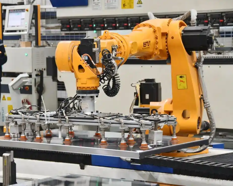
1. Problem Analysis in Conventional Cooperative Systems
In a conventional automation cell, the PLC and the industrial robot controller usually communicate through a gateway, a serial link, or a general-purpose Ethernet protocol. The PLC executes cyclic logic, while the industrial robot executes a motion program. When the PLC needs to send a Cartesian target pose to the industrial robot, the data may be converted into ASCII strings, packed into Modbus registers, or transferred through a proprietary function block. Each conversion step adds processing time, and each polling cycle adds waiting time. The result is a communication path that may be acceptable for simple material handling but is inadequate for high-dynamic tasks such as laser welding, precision dispensing, or force-controlled assembly.
I decompose the total communication delay into several components. Let \(L_{\text{total}}\) be the end-to-end latency between the PLC application layer and the industrial robot application layer. Then:
$$L_{\text{total}} = L_{\text{proc}} + L_{\text{stack}} + L_{\text{trans}} + L_{\text{wait}} + L_{\text{jitter}}$$
Here, \(L_{\text{proc}}\) is the application processing time in the PLC and the industrial robot controller, \(L_{\text{stack}}\) is the protocol stack traversal time, \(L_{\text{trans}}\) is the physical transmission time, \(L_{\text{wait}}\) is the polling or scheduling wait time, and \(L_{\text{jitter}}\) is the stochastic variation caused by network congestion, interrupt latency, or operating system scheduling. In a Modbus TCP polling system, \(L_{\text{wait}}\) often dominates because the master must poll the slave at a fixed interval. If the polling interval is 10 ms and the industrial robot needs six degrees of freedom, the effective update rate may fall below 100 Hz. In contrast, a Profinet real-time channel can achieve a cycle time of 2 ms to 8 ms with bounded jitter.
For a serial ASCII link, the transmission time is also significant. If a target pose is encoded as \(N_{\text{char}}\) characters, each character uses \(N_{\text{bits}}\) bits, and the baud rate is \(R_{\text{baud}}\), then the raw transmission time is:
$$T_{\text{serial}} = \frac{N_{\text{char}} \cdot N_{\text{bits}}}{R_{\text{baud}}}$$
For example, with 120 characters, 10 bits per character, and a 115200 baud link, \(T_{\text{serial}}\) is approximately 10.4 ms before any parsing or interpolation. If the industrial robot must receive a new pose every 4 ms, this link is fundamentally insufficient. The problem is not only bandwidth but also determinism. A general-purpose TCP/IP stack may retransmit lost packets, coalesce segments, or delay acknowledgments, all of which are harmful to motion control.
Table 1 summarizes the communication characteristics I typically observe in heterogeneous cells. The comparison is not intended to declare one protocol universally superior, but to show why a real-time industrial Ethernet approach is necessary for tight coordination between industrial robots and PLCs.
| Communication Method | Typical Cycle Time | Jitter | Data Granularity | Suitability for Industrial Robots and PLCs |
|---|---|---|---|---|
| Serial ASCII | 10-50 ms | High | Character-based | Low: parameter transfer only |
| Modbus TCP polling | 10-30 ms | Medium to high | Register-based | Limited: slow sequencing |
| Profinet RT | 4-10 ms | Low | Cyclic I/O | Good: coordinated motion |
| Profinet IRT | 0.25-4 ms | Very low | Cyclic and isochronous | Excellent: high-precision sync |
| EtherCAT | 0.1-2 ms | Very low | Distributed clocks | Excellent: multi-axis motion |
| EtherNet/IP with CIP Sync | 1-10 ms | Low | Implicit and explicit | Good: discrete and motion |
The second major problem is control logic. Many existing cells use a master-request/slave-response sequence. The PLC sends a command, the industrial robot executes it, the industrial robot returns a completion flag, and only then does the PLC send the next command. This pattern is easy to program and debug, but it creates dead time between motions. If the industrial robot accelerates, decelerates, and waits for a handshake at every waypoint, the average velocity is much lower than the mechanical capability of the industrial robot. I model the wasted time as:
$$T_{\text{waste}} = \sum_{i=1}^{M} \left( T_{\text{handshake},i} + T_{\text{settle},i} \right)$$
where \(M\) is the number of sequential steps, \(T_{\text{handshake},i}\) is the communication and logic delay for step \(i\), and \(T_{\text{settle},i}\) is the mechanical settling time. In a typical pick-and-place cycle with 12 steps, even 8 ms of handshake delay per step adds nearly 100 ms to the cycle. For an industrial robot performing 60 cycles per minute, this is a serious loss. The solution is not to remove all handshakes, because safety and process constraints still require confirmation, but to overlap communication with motion and to use time-stamped commands so that the industrial robot can plan its trajectory continuously.
2. Profinet-Based Physical and Protocol Architecture
I selected Profinet as the backbone because it supports both standard TCP/IP communication and real-time cyclic data exchange. Profinet real-time class 1 is suitable for general automation, while Profinet isochronous real time is suitable for motion synchronization between industrial robots, servo drives, and distributed I/O. The protocol bypasses the standard TCP/IP stack for cyclic data, which reduces \(L_{\text{stack}}\) and \(L_{\text{jitter}}\). In my architecture, the PLC acts as the Profinet controller, and each industrial robot controller acts as a Profinet device. A General Station Description file is imported into the PLC engineering tool, and the robot interface is mapped into the PLC input and output address space. This hardware-level integration means that reading a robot status word is as straightforward as reading a local variable.
The physical topology can be star, line, or ring depending on the cell layout. I prefer a star topology with an industrial managed switch for high availability, combined with a line topology for distributed I/O near the industrial robots. The PLC, robot controllers, servo drives, vision system, and remote I/O modules are connected through the switch. The network design must respect the following constraints:
$$T_{\text{cycle}} = T_{\text{io}} + T_{\text{net}} + T_{\text{switch}} + T_{\text{jitter}} \leq T_{\text{required}}$$
where \(T_{\text{cycle}}\) is the actual Profinet cycle, \(T_{\text{io}}\) is the device I/O processing time, \(T_{\text{net}}\) is the cable propagation time, \(T_{\text{switch}}\) is the store-and-forward delay, and \(T_{\text{required}}\) is the maximum allowable cycle for the application. For precision assembly with industrial robots, I set \(T_{\text{required}}\) to 4 ms or less. For welding and dispensing, 8 ms may be sufficient, but I still prefer 4 ms to provide margin.
Table 2 lists the network parameters I use in a typical flexible assembly cell. These values are not universal constants, but they represent a practical baseline for Profinet IRT deployment with industrial robots.
| Parameter | Value | Description |
|---|---|---|
| Profinet class | IRT | Isochronous real time for motion |
| Cycle time | 2-4 ms | Deterministic update period |
| Jitter | < 1 μs | Hardware-supported synchronization |
| Topology | Star and line | Managed switch and distributed devices |
| Number of industrial robots | 1-6 | Scalable to multi-robot cells |
| Remote I/O | ET200SP class | Distributed safety and standard I/O |
| Vision integration | Profinet or TCP/IP | Result and image trigger channels |
| Safety protocol | PROFIsafe | Functional safety over Profinet |
The PLC controller in my design performs global logic scheduling, external I/O management, safety interlocking, and process sequencing. The industrial robot controller performs motion planning, inverse kinematics, trajectory interpolation, and servo control. I do not attempt to make the PLC perform robot interpolation, because that would overload the PLC scan cycle and duplicate functions that the robot controller already executes well. Instead, the PLC sends high-level commands and time-stamped targets, and the industrial robot controller executes them with its native motion planner. This division of labor preserves the strengths of both systems.
3. Block Data Transmission and Shared Memory Mapping
Single-word read and write operations are inefficient for cooperative motion. A six-degree-of-freedom pose requires six real values, plus control words, task indices, process parameters, and heartbeat counters. If the PLC writes each value separately, the industrial robot may observe an inconsistent set of values during the update. I therefore use block data transmission with two shared memory areas: a PLC-to-robot block and a robot-to-PLC block. Both blocks are mapped into the Profinet cyclic I/O image. The PLC writes the entire output block in one consistent snapshot, and the industrial robot reads the entire input block in one consistent snapshot.
Let \(B_{\text{P2R}}\) be the PLC-to-robot block and \(B_{\text{R2P}}\) be the robot-to-PLC block. The data consistency condition is:
$$B_{\text{P2R}}(k) = \left\{ C(k), I(k), P(k), Q(k), H(k) \right\}$$
where \(k\) is the communication cycle index, \(C(k)\) is the control word, \(I(k)\) is the task index, \(P(k)\) is the target pose, \(Q(k)\) is the process parameter set, and \(H(k)\) is the heartbeat counter. The industrial robot only updates its internal command buffer when the entire block \(B_{\text{P2R}}(k)\) is received and validated. Similarly, the PLC only updates its status variables when the entire block \(B_{\text{R2P}}(k)\) is received and validated. This snapshot mechanism prevents data tearing and ensures that multi-dimensional commands are applied atomically.
Table 3 defines the PLC-to-robot block I use. The total length is 64 bytes, which fits comfortably within a typical Profinet cyclic frame and leaves room for future expansion.
| Byte Offset | Data Name | Length (Bytes) | Data Type | Function |
|---|---|---|---|---|
| 00-01 | Control word | 2 | WORD | Start, stop, reset, pause, and mode bits |
| 02-03 | Task index | 2 | UINT | Process program number |
| 04-27 | Target pose | 24 | REAL[6] | X, Y, Z, A, B, C |
| 28-39 | Process parameters | 12 | REAL[3] | Speed, power, pressure, or flow |
| 40-61 | Reserved extension | 22 | BYTE[22] | Future sensor and configuration data |
| 62-63 | Heartbeat | 2 | UINT | Link liveness counter |
Table 4 defines the robot-to-PLC block. It includes the robot status, current pose, joint positions, torque feedback, safety state, and diagnostic codes. The torque feedback is important for collision detection and adaptive process control.
| Byte Offset | Data Name | Length (Bytes) | Data Type | Function |
|---|---|---|---|---|
| 00-01 | Status word | 2 | WORD | Ready, busy, done, error, safety |
| 02-03 | Active task index | 2 | UINT | Currently executing program |
| 04-27 | Actual pose | 24 | REAL[6] | Measured Cartesian pose |
| 28-51 | Joint positions | 24 | REAL[6] | Encoder or model-based joint angles |
| 52-63 | Torque feedback | 12 | REAL[3] | Representative axis torques |
| 64-65 | Safety state | 2 | WORD | Safe stop, protective stop, normal |
| 66-67 | Diagnostic code | 2 | UINT | Fault and warning codes |
| 68-69 | Heartbeat echo | 2 | UINT | Returned heartbeat value |
The block transmission efficiency can be expressed as:
$$\eta_{\text{block}} = \frac{N_{\text{payload}}}{N_{\text{payload}} + N_{\text{overhead}}} \times 100\%$$
For a 64-byte payload with 12 bytes of Profinet cyclic overhead, \(\eta_{\text{block}}\) is about 84%. In contrast, a single-register Modbus TCP transaction may carry only 2 bytes of payload with 10-20 bytes of overhead, yielding an efficiency below 15%. The block approach also reduces the number of transactions. If the PLC needs 20 values, a single block transfer replaces 20 separate reads or writes. This reduces CPU load on both the PLC and the industrial robot controller, and it lowers the probability of scheduling conflicts.
4. Master-Slave Control Logic and Timestamp Synchronization
I use the PLC as the master for global logic and the industrial robot as the slave for motion execution. However, the word “slave” does not mean that the industrial robot waits passively for every micro-step. The PLC sends a target pose with a timestamp, and the industrial robot plans a continuous trajectory to reach that pose at the specified time. This is a time-driven control strategy rather than a request-response strategy. The industrial robot can interpolate through multiple PLC cycles without stopping, which preserves motion continuity and reduces vibration.
Let \(T_{\text{send}}\) be the PLC timestamp when the command is generated, \(T_{\text{recv}}\) be the industrial robot receive timestamp, \(T_{\text{buffer}}\) be a configured buffering window, and \(\Delta t\) be the measured one-way delay. The industrial robot computes the desired action time as:
$$T_{\text{action}} = T_{\text{recv}} + T_{\text{buffer}} – \Delta t$$
The delay estimate is:
$$\Delta t = T_{\text{recv}} – T_{\text{send}}$$
The buffer window \(T_{\text{buffer}}\) is typically set to 2 to 4 communication cycles. If the cycle time is 2 ms, \(T_{\text{buffer}}\) is 4 to 8 ms. This window absorbs small network jitter and allows the industrial robot to plan a smooth trajectory. If the jitter exceeds the buffer, the industrial robot can reduce speed or hold position, depending on the safety state. The time-stamped command also allows the PLC to coordinate an external axis, such as a positioner or a linear track, with the industrial robot. Both devices receive the same time base and execute their motions in a synchronized time window.
Table 5 lists the timing parameters I use in a representative multi-robot cell. The values are chosen to balance responsiveness and robustness. A smaller buffer improves reaction time but increases the risk of underflow during network congestion. A larger buffer improves robustness but adds phase lag. I tune the buffer according to the process: welding and dispensing can tolerate more buffering, while assembly and inspection require tighter synchronization.
| Parameter | Symbol | Value | Effect |
|---|---|---|---|
| Profinet cycle | \(T_{\text{cycle}}\) | 2 ms | Base update period |
| Buffer window | \(T_{\text{buffer}}\) | 4-8 ms | Absorbs jitter |
| Timestamp resolution | \(T_{\text{res}}\) | 1 μs | Fine synchronization |
| Maximum jitter | \(J_{\max}\) | < 1 μs | IRT hardware support |
| Trajectory interpolation period | \(T_{\text{interp}}\) | 1 ms | Robot internal motion planner |
| PLC scan time | \(T_{\text{scan}}\) | 1-2 ms | Logic execution |
| Safety reaction time | \(T_{\text{safety}}\) | < 10 ms | PROFIsafe and drive shutdown |
The timestamp synchronization error can be modeled as:
$$e_{\text{sync}} = \left( T_{\text{recv}} – T_{\text{send}} \right) – \Delta t_{\text{true}} + \epsilon_{\text{clock}}$$
where \(\Delta t_{\text{true}}\) is the true propagation delay and \(\epsilon_{\text{clock}}\) is the clock offset between the PLC and the industrial robot controller. Profinet IRT provides hardware-based clock synchronization, so \(\epsilon_{\text{clock}}\) is in the sub-microsecond range. If standard Ethernet is used, \(\epsilon_{\text{clock}}\) may reach several milliseconds, which is unacceptable for coordinated motion. This is one reason I insist on IRT or an equivalent synchronized Ethernet solution for multi-axis cooperation.
The trajectory tracking error caused by communication jitter can be approximated as:
$$e_{\text{track}} = v_{\max} \cdot J_{\text{eff}}$$
where \(v_{\max}\) is the maximum path velocity and \(J_{\text{eff}}\) is the effective timing jitter. For a welding speed of 100 mm/s and a jitter of 1 ms, \(e_{\text{track}}\) is 0.1 mm. For a high-speed assembly motion at 500 mm/s, the same jitter produces 0.5 mm of error. This shows why deterministic communication is not optional for industrial robots that perform precision work.
5. Exception Handling, Heartbeat Monitoring, and Safety Interlock
Industrial environments contain electromagnetic interference, network congestion, cable faults, and power disturbances. A cooperative system must detect communication failures quickly and transition to a safe state. I use a heartbeat counter in both shared memory blocks. The PLC increments its heartbeat every cycle and writes it to the PLC-to-robot block. The industrial robot copies the received heartbeat into the robot-to-PLC block. The PLC then compares the returned heartbeat with its expected value. If the difference persists for several cycles, the PLC declares a communication fault.
Let \(C_{\text{heartbeat}}(k)\) be the PLC heartbeat at cycle \(k\), and let \(N\) be the number of tolerated missing or mismatched cycles. The link state function is:
$$S_{\text{link}}(k) =
\begin{cases}
1, & \sum_{i=0}^{N-1} \left| C_{\text{heartbeat}}(k-i) – C_{\text{heartbeat}}(k-i-1) \right| = N \\
0, & \text{otherwise}
\end{cases}$$
In my implementation, \(N\) is set to 5. With a 4 ms cycle, this corresponds to a detection window of about 20 ms. If \(S_{\text{link}}(k)=0\), the system triggers a soft emergency stop. The industrial robot does not cut power immediately, because an abrupt power loss on a moving industrial robot can cause mechanical shock or loss of holding torque. Instead, the industrial robot performs a controlled deceleration along the current path and then enters a safe stop state. The PLC disables process outputs, such as welding power, adhesive flow, or tool activation, and raises an alarm. This layered response protects both the equipment and the workpiece.
Table 6 summarizes the safety states and transitions I use. The transition logic is implemented partly in the PLC and partly in the industrial robot controller, with PROFIsafe carrying safety-related signals.
| State | Trigger | PLC Action | Industrial Robot Action |
|---|---|---|---|
| Normal | \(S_{\text{link}}=1\), no fault | Run process logic | Track trajectory |
| Warning | Single heartbeat mismatch | Log event, continue | Continue with monitoring |
| Soft stop | \(S_{\text{link}}=0\) | Disable process outputs | Controlled deceleration |
| Protective stop | Safety input active | Drop safety relay | Safe torque off |
| Emergency stop | E-stop button pressed | Cut power to drives | Mechanical brake engagement |
| Recovery | Fault cleared and reset | Reinitialize communication | Re-home or resume |
Beyond communication faults, I also monitor collision and overload conditions. The industrial robot controller provides current feedback for each axis. I estimate the external torque residual by comparing the measured torque with a model-based reference. Let \(K_t\) be the motor torque constant, \(I_{\text{fb}}\) be the measured current, \(J\) be the equivalent inertia, \(B\) be the viscous friction coefficient, \(\theta\) be the joint angle, \(\dot{\theta}\) be the joint velocity, \(\ddot{\theta}\) be the joint acceleration, and \(T_{\text{load}}\) be the modeled load torque. The collision residual is:
$$R_{\text{collision}} = K_t I_{\text{fb}} – \left( J \ddot{\theta} + B \dot{\theta} + T_{\text{load}} \right)$$
If \(|R_{\text{collision}}|\) exceeds a threshold \(\tau_{\text{collision}}\) for a specified time, the industrial robot declares a collision. The threshold can be fixed or adaptive:
$$\tau_{\text{collision}} = \tau_0 + \alpha \left\| \dot{\theta} \right\| + \beta \left\| \ddot{\theta} \right\|$$
where \(\tau_0\) is a base threshold, \(\alpha\) and \(\beta\) are velocity and acceleration weighting factors. This adaptive threshold reduces false positives during high-speed motion while remaining sensitive to unexpected contact at low speed. I send the collision state to the PLC through the robot-to-PLC block, and the PLC disables the process and commands a safe stop.
Table 7 lists representative threshold values for a medium-payload industrial robot. These values must be tuned for each mechanical configuration, payload, and process.
| Parameter | Value | Unit | Purpose |
|---|---|---|---|
| Base threshold \(\tau_0\) | 5.0 | N·m | Low-speed collision detection |
| Velocity weight \(\alpha\) | 0.15 | N·m·s/rad | Compensate for speed-dependent friction |
| Acceleration weight \(\beta\) | 0.05 | N·m·s²/rad | Compensate for inertial modeling error |
| Collision time window | 10 | ms | Avoid transient false alarms |
| Heartbeat tolerance \(N\) | 5 | cycles | Detect link loss within 20 ms |
| Soft stop deceleration | 0.3 | m/s² | Controlled stop without shock |
6. Experimental Platform and Communication Performance
I built an experimental platform to validate the proposed communication optimization and control strategy. The platform consists of a PLC with Profinet IRT support, a six-axis industrial robot, a servo positioner, a laser vision sensor, and a remote I/O station. The PLC is the Profinet controller, and the industrial robot, positioner, and remote I/O are Profinet devices. The vision sensor communicates through a separate Gigabit Ethernet channel for image data but synchronizes its trigger and result signals through Profinet. I also introduced controlled electromagnetic interference and network traffic to test robustness.
Table 8 lists the main hardware components. The exact vendor names are not important for the methodology, but the functional roles are.
| Component | Role | Interface | Key Feature |
|---|---|---|---|
| PLC | Master controller | Profinet IRT | 1 ms scan, 2 ms cycle |
| Industrial robot | Motion slave | Profinet device | Six axes, 1 ms interpolation |
| Servo positioner | External axis | Profinet IRT | Synchronized with robot |
| Remote I/O | Distributed signals | Profinet RT | Standard and safety I/O |
| Vision sensor | Guidance and inspection | Gigabit Ethernet | Trigger and result over Profinet |
| Managed switch | Network infrastructure | Industrial Ethernet | QoS and diagnostics |
| Safety controller | Functional safety | PROFIsafe | Safe stop and monitoring |
I compared two configurations. The baseline configuration used Modbus TCP polling with a 10 ms polling interval and ASCII-encoded pose data. The optimized configuration used Profinet IRT with block data transmission, shared memory mapping, timestamp synchronization, and heartbeat monitoring. I ran each configuration for 24 hours and collected more than \(10^7\) data packets. The metrics were average round-trip latency, latency jitter, packet loss rate, and cooperative trajectory error.
Table 9 shows the aggregated results. The optimized configuration reduced the average round-trip latency from 15.2 ms to 3.8 ms, a reduction of about 75%. The jitter decreased from ±4.5 ms to ±0.4 ms. The packet loss rate fell from 0.120% to less than 0.001%. The cooperative trajectory error, measured as the maximum deviation between the commanded path and the actual path during a coordinated motion, decreased from 2.40 mm to 0.35 mm.
| Metric | Baseline (Modbus TCP) | Optimized (Profinet IRT + Block Transfer) | Improvement |
|---|---|---|---|
| Average round-trip latency | 15.2 ms | 3.8 ms | 75.0% lower |
| Latency jitter | ±4.5 ms | ±0.4 ms | 91.1% lower |
| Packet loss rate | 0.120% | < 0.001% | > 99.2% lower |
| Cooperative trajectory error | 2.40 mm | 0.35 mm | 85.4% lower |
| Effective command rate | ≈ 66 Hz | ≈ 250 Hz | 3.8× higher |
| Motion stop time per cycle | 80-120 ms | 0-10 ms | Near elimination |
The percentage improvement is calculated as:
$$\text{Improvement} = \frac{X_{\text{baseline}} – X_{\text{optimized}}}{X_{\text{baseline}}} \times 100\%$$
For latency, this gives:
$$\frac{15.2 – 3.8}{15.2} \times 100\% = 75.0\%$$
For trajectory error:
$$\frac{2.40 – 0.35}{2.40} \times 100\% = 85.4\%$$
The effective command rate is the reciprocal of the average round-trip latency:
$$f_{\text{cmd}} = \frac{1}{L_{\text{total}}}$$
For the optimized system, \(f_{\text{cmd}} \approx 263\) Hz, which is limited by the Profinet cycle and robot interpolation. I report 250 Hz as a conservative value. This rate is sufficient for dynamic welding, dispensing, and assembly tasks performed by industrial robots.
I also measured the synchronization error between the industrial robot and the external positioner. Table 10 shows the results for three motion profiles: slow contouring, medium-speed assembly, and high-speed transfer. The synchronization error is defined as the maximum difference between the commanded and actual phase angle during coordinated motion.
| Motion Profile | Path Speed | Baseline Sync Error | Optimized Sync Error | Improvement |
|---|---|---|---|---|
| Slow contouring | 20 mm/s | 1.10 mm | 0.12 mm | 89.1% |
| Medium assembly | 120 mm/s | 1.85 mm | 0.22 mm | 88.1% |
| High-speed transfer | 500 mm/s | 3.60 mm | 0.48 mm | 86.7% |
| Welding weave | 60 mm/s | 1.40 mm | 0.18 mm | 87.1% |
The contour error for a three-dimensional path is computed as:
$$e_{\text{contour}} = \sqrt{e_x^2 + e_y^2 + e_z^2}$$
where \(e_x\), \(e_y\), and \(e_z\) are the axis-wise deviations from the commanded path. In the optimized system, the maximum contour error remains below 0.35 mm for the tested profiles. This is within the tolerance for many industrial robots used in arc welding, adhesive dispensing, and light assembly. For higher precision, additional compensation or external metrology may be required, but the communication and timing foundation is already in place.
7. Control Strategy Performance and Multi-Robot Coordination
The control strategy is not limited to a single industrial robot. I extended the architecture to two industrial robots and one positioner. The PLC coordinates the group by assigning time-stamped targets and by monitoring shared safety states. Each industrial robot executes its own trajectory, but the PLC ensures that their motions do not collide and that their process actions occur in the correct order. The shared memory model is extended with a coordination block that contains the group state, the active robot mask, and the synchronization barrier counter.
Let \(G(k)\) be the group coordination state at cycle \(k\). The PLC computes:
$$G(k) = \bigwedge_{j=1}^{R} S_{\text{ready},j}(k) \land S_{\text{safe}}(k) \land S_{\text{link}}(k)$$
where \(R\) is the number of industrial robots, \(S_{\text{ready},j}(k)\) is the ready state of robot \(j\), \(S_{\text{safe}}(k)\) is the cell safety state, and \(S_{\text{link}}(k)\) is the communication link state. The group motion is allowed only when all robots are ready, the cell is safe, and the communication link is healthy. This logical conjunction prevents a partially ready robot from being commanded into a coordinated motion.
Table 11 shows the coordination performance for a two-robot assembly task. The task involves one industrial robot presenting a part and another industrial robot fastening it, while a positioner rotates the fixture. The cycle time, synchronization error, and success rate are compared between the baseline and optimized systems.
| Metric | Baseline | Optimized | Change |
|---|---|---|---|
| Cycle time | 8.6 s | 6.1 s | 29.1% shorter |
| Maximum sync error | 2.2 mm | 0.30 mm | 86.4% lower |
| Task success rate | 94.2% | 99.6% | 5.4 percentage points higher |
| Unexpected stops per 1000 cycles | 12.4 | 1.1 | 91.1% fewer |
| Average PLC CPU load | 38% | 42% | 4 percentage points higher |
| Average network utilization | 21% | 34% | 13 percentage points higher |
The PLC CPU load and network utilization increase slightly because the optimized system exchanges more data per cycle. However, the increase is acceptable and remains well below the capacity limits. The reduction in unexpected stops is particularly important for production availability. In the baseline system, many stops were caused by polling timeouts and inconsistent data. In the optimized system, the heartbeat and snapshot mechanisms detect true faults quickly while avoiding false alarms.
I further evaluated the control strategy under induced disturbances. I injected burst errors, increased switch traffic, and temporarily blocked one Profinet device. The optimized system detected the fault within 20 ms and entered a soft stop. The baseline system sometimes continued with stale data for more than 100 ms, which is dangerous for cooperative motion. This confirms that communication optimization is not only a performance improvement but also a safety function.
8. Comparison with Alternative Industrial Ethernet Approaches
Although I selected Profinet for this implementation, the methodology can be adapted to other industrial Ethernet protocols. EtherCAT offers very low cycle times and distributed clocks, which are excellent for multi-axis motion. EtherNet/IP with CIP Sync provides good integration with CIP-based devices. SERCOS III provides deterministic motion control for servo drives. The key requirements are the same: cyclic data exchange, time synchronization, block data mapping, and safety interlock. Table 12 compares these protocols from the perspective of industrial robot and PLC cooperation.
| Protocol | Typical Cycle | Time Sync | Robot Integration | PLC Integration | Notes |
|---|---|---|---|---|---|
| Profinet IRT | 0.25-4 ms | Hardware | Wide vendor support | Strong in Siemens ecosystems | Excellent for coordinated motion |
| EtherCAT | 0.1-2 ms | Distributed clocks | Common in motion control | Requires compatible master | Very low jitter |
| EtherNet/IP + CIP Sync | 1-10 ms | IEEE 1588 | Wide vendor support | Strong in Rockwell ecosystems | Good for discrete and motion |
| SERCOS III | 0.125-1 ms | Hardware | Motion-centric | Specialized | High performance for drives |
| Modbus TCP | 10-30 ms | None | Gateway required | Simple | Not suitable for tight motion |
| OPC UA Pub/Sub | 1-10 ms | TSN optional | Growing support | Growing support | Good for data integration |
My choice of Profinet was driven by the need to integrate a PLC-based cell with industrial robots from multiple vendors and to use a single engineering environment for both logic and motion coordination. The block data and timestamp concepts are protocol-independent. If I were to use EtherCAT, I would map the shared memory to EtherCAT process data and use distributed clocks for synchronization. If I were to use OPC UA Pub/Sub with TSN, I would use time-sensitive networking for deterministic delivery and OPC UA information models for semantic data. The control strategy would remain similar.
9. Practical Implementation Considerations
Several practical details affect the success of the proposed approach. First, the Profinet device description file must correctly define the input and output modules, the data lengths, and the consistency over the entire block. If the consistency is set to one byte instead of one block, the snapshot mechanism may fail. Second, the PLC and industrial robot must agree on endianness and data alignment. A REAL value in the PLC may be big-endian or little-endian depending on the platform, and the industrial robot may expect a different byte order. I use a documented mapping and a commissioning test that writes known values to the shared memory and reads them back.
Third, the heartbeat and safety logic must be designed so that a single point of failure does not cause an unsafe state. The heartbeat is not a substitute for a safety-rated protocol. I use PROFIsafe for safety-related signals and treat the heartbeat as a diagnostic and coordination mechanism. The safety-rated signals include emergency stop, protective door, enabling device, and safe torque off. These signals are transmitted over the same physical network but with safety protocol layers that meet the required performance level.
Fourth, the time buffer must be tuned. A buffer that is too small causes frequent underflow and speed reduction. A buffer that is too large increases the response time to process changes. I typically start with \(T_{\text{buffer}} = 3 T_{\text{cycle}}\) and adjust based on measured jitter. If the measured jitter is \(J_{99}\) (99th percentile), I require:
$$T_{\text{buffer}} \geq J_{99} + T_{\text{margin}}$$
where \(T_{\text{margin}}\) is a safety margin of at least one cycle. For a stable Profinet IRT network, \(J_{99}\) is below 1 μs, so the buffer is dominated by the desired response time rather than by jitter. For a network with standard Ethernet traffic, \(J_{99}\) may be several milliseconds, and the buffer must be larger or the network must be segmented.
Fifth, the industrial robot controller must support external time-stamped commands. Some industrial robots accept only simple start/stop signals or proprietary motion commands. In that case, I use a robot-specific interface function that converts the block data into the native command format. If the industrial robot does not support time-stamped targets, I implement a trajectory streaming mode in which the PLC sends a new setpoint every cycle, and the industrial robot uses a low-level servo interface. This requires a high-performance controller and a well-tuned feedforward loop, but it can achieve excellent synchronization.
10. Mathematical Modeling of the Cooperative Control Loop
To analyze the stability of the cooperative control loop, I model the PLC and the industrial robot as a discrete-time system. Let \(x(k)\) be the robot state, \(u(k)\) be the command from the PLC, and \(y(k)\) be the measured output. The state-space representation is:
$$x(k+1) = A x(k) + B u(k) + w(k)$$
$$y(k) = C x(k) + v(k)$$
where \(A\) is the state transition matrix, \(B\) is the input matrix, \(C\) is the output matrix, \(w(k)\) is the process noise, and \(v(k)\) is the measurement noise. The PLC controller computes the command based on the reference \(r(k)\) and the feedback \(y(k)\):
$$u(k) = K_p e(k) + K_i \sum_{i=0}^{k} e(i) + K_d \left( e(k) – e(k-1) \right)$$
where \(e(k) = r(k) – y(k)\). In the optimized system, the feedback delay is small and bounded, so the controller gains can be increased without causing instability. The closed-loop characteristic equation is:
$$\det \left( zI – A + B K \right) = 0$$
where \(K\) is the combined controller gain. If the delay exceeds one or more sampling periods, the effective plant model must include a delay term \(z^{-d}\), and the stability margin decreases. The communication optimization reduces \(d\) and thus improves the achievable bandwidth. This is a key reason why deterministic communication enables higher control performance for industrial robots.
I also model the synchronization error between two industrial robots. Let \(e_1(k)\) and \(e_2(k)\) be their tracking errors. The relative error is:
$$e_{\text{rel}}(k) = e_1(k) – e_2(k)$$
The variance of the relative error is:
$$\sigma_{\text{rel}}^2 = \sigma_1^2 + \sigma_2^2 – 2 \rho \sigma_1 \sigma_2$$
where \(\sigma_1^2\) and \(\sigma_2^2\) are the individual error variances, and \(\rho\) is the correlation coefficient. When both industrial robots share the same time base and receive synchronized commands, \(\rho\) increases, and \(\sigma_{\text{rel}}^2\) decreases. This mathematical result supports the use of a common time-stamped control strategy.
11. Data Analysis and Statistical Evaluation
I performed statistical analysis on the latency measurements. The latency distribution in the baseline system is heavy-tailed, with occasional spikes beyond 50 ms. The optimized system has a narrow distribution centered at 3.8 ms. I compute the mean, standard deviation, and 99th percentile as follows:
$$\mu = \frac{1}{N} \sum_{i=1}^{N} L_i$$
$$\sigma = \sqrt{\frac{1}{N-1} \sum_{i=1}^{N} \left( L_i – \mu \right)^2}$$
$$L_{99} = \text{percentile}(L, 99)$$
Table 13 shows the latency statistics for both configurations. The optimized system has a much lower \(L_{99}\), which is critical for worst-case motion performance. A low average latency is not enough if the worst-case latency causes a trajectory deviation or a missed synchronization window.
| Statistic | Baseline (ms) | Optimized (ms) | Improvement |
|---|---|---|---|
| Mean \(\mu\) | 15.2 | 3.8 | 75.0% |
| Standard deviation \(\sigma\) | 4.5 | 0.4 | 91.1% |
| 99th percentile \(L_{99}\) | 42.0 | 5.1 | 87.9% |
| Maximum observed | 88.0 | 6.2 | 93.0% |
| Minimum observed | 8.0 | 3.1 | 61.3% |
The maximum observed latency in the optimized system is 6.2 ms, which is only slightly above the mean. This bounded behavior is the result of Profinet IRT scheduling and the block transfer mechanism. In the baseline system, the maximum latency is more than five times the mean, which makes worst-case design difficult. For industrial robots performing safety-critical or high-value processes, bounded latency is more important than average latency.
12. Scalability and Future Extensions
The proposed architecture scales to additional industrial robots, external axes, and sensors. Each new Profinet device adds cyclic data to the network, so the network load must be calculated. Let \(N_d\) be the number of devices, \(S_i\) be the data size of device \(i\) in bytes, and \(T_{\text{cycle}}\) be the cycle time. The approximate network utilization is:
$$U = \frac{\sum_{i=1}^{N_d} S_i \cdot 8}{T_{\text{cycle}} \cdot R_{\text{link}}} \times 100\%$$
where \(R_{\text{link}}\) is the link rate in bits per second. For a 100 Mbit/s link with 6 devices, 64 bytes per device, and a 2 ms cycle, the utilization is:
$$U = \frac{6 \cdot 64 \cdot 8}{0.002 \cdot 100 \times 10^6} \times 100\% \approx 15.4\%$$
This leaves ample capacity for vision results, diagnostics, and future expansion. For larger cells, I recommend a Gigabit backbone and segmented network domains. I also recommend separating safety traffic, motion traffic, and best-effort traffic using VLANs or Profinet priorities.
Future extensions include time-sensitive networking, edge computing, and cloud analytics. TSN can provide deterministic Ethernet for mixed traffic, which is useful when industrial robots, PLCs, cameras, and IT systems share the same infrastructure. Edge computing can run advanced control algorithms, such as model predictive control or vision-based servoing, near the industrial robots. Cloud analytics can monitor long-term performance and predict maintenance needs. Table 14 summarizes potential extensions and their expected impact.
| Extension | Benefit | Challenge | Applicability to Industrial Robots and PLCs |
|---|---|---|---|
| TSN | Deterministic mixed traffic | Configuration complexity | High |
| Edge control | Lower latency for advanced algorithms | Hardware cost | High |
| OPC UA Pub/Sub | Semantic data integration | Maturity of motion profiles | Medium to high |
| Digital twin | Simulation and commissioning | Model accuracy | High |
| AI-based anomaly detection | Predictive maintenance | Data quality and labeling | Medium to high |
| 5G private networks | Flexible mobile robots | Determinism and coverage | Medium |
I am particularly interested in combining the timestamp synchronization strategy with a digital twin. If the PLC and the industrial robot share a common time base, the digital twin can replay the exact motion and communication sequence for diagnostics. The twin can also predict the effect of communication jitter on path accuracy and suggest buffer settings. This closes the loop between design, operation, and optimization.
13. Limitations and Risk Mitigation
The proposed approach has limitations. It assumes that the industrial robot controller supports Profinet or a comparable real-time protocol. If the industrial robot is older or uses a closed proprietary interface, a gateway may be required, and the gateway may reintroduce latency. In that case, I recommend using the fastest available gateway and placing it as close as possible to the robot controller. I also recommend measuring the gateway latency and including it in the control design.
The approach also assumes that the network is properly engineered. Poor cable routing, unmanaged switches, and excessive broadcast traffic can destroy determinism. I mitigate these risks by using managed industrial switches, shielded cables, proper grounding, and network segmentation. I also monitor network statistics through the PLC and trigger a warning if the cycle time or jitter exceeds a threshold.
Another limitation is that the collision detection model depends on accurate dynamic parameters. If the payload changes or the robot wears over time, the residual threshold may need adjustment. I use adaptive thresholding and periodic model identification to reduce false positives and false negatives. The collision detection is not a substitute for safety-rated force limiting, but it provides an additional layer of protection for industrial robots.
14. Conclusion
I have presented a communication optimization and control strategy for industrial robots and PLCs operating in a cooperative cell. The strategy uses Profinet IRT for deterministic communication, block data transmission for efficient and consistent data exchange, shared memory mapping for atomic updates, timestamp synchronization for coordinated motion, heartbeat monitoring for link health, and collision residual analysis for safety. The experimental results show a 75% reduction in average round-trip latency, a 91% reduction in jitter, and an 85% reduction in cooperative trajectory error. The optimized system achieves an effective command rate of approximately 250 Hz and maintains synchronization errors below 0.35 mm in the tested profiles.
The broader lesson is that communication is not a background detail in industrial robot and PLC cooperation. It is a first-class design variable that determines motion accuracy, cycle time, safety, and scalability. By treating the PLC and the industrial robot as a single time-coordinated system, I can achieve performance that is not possible with request-response polling or serial links. The proposed methods are protocol-adaptable and can be applied to EtherCAT, EtherNet/IP with CIP Sync, SERCOS III, or future TSN-based architectures. As manufacturing moves toward higher flexibility and intelligence, deterministic communication and time-aware control will remain essential foundations for industrial robots and PLCs working together.
In future work, I plan to extend the shared memory model to include semantic process data, integrate OPC UA Pub/Sub over TSN, and evaluate the control strategy with mobile industrial robots and reconfigurable fixtures. I also plan to study the interaction between communication jitter and advanced model predictive control, because the next generation of industrial robots will need both high precision and high adaptability. The results presented here provide a practical and extensible baseline for those efforts.